Newbie as a data scientist in East Asia! (kaggle Competition)
Newbie as a data scientist in East Asia!
Hello, Kaggers! Nice to meet you!
We are a team in East Asia that wants to be data scientists
As newbies, we want to know what and/or how Kaggler is!
so, let’s have a time to learn about Kaggle as a senior with us from now.
If you want to support us (or feel qute) , I ask for a comment! (PLZ) ^0^
And !! Since we are not native English speakers, please ask questions if there is a context that you don’t understand because it’s not smooth.
I’ll do my best to answer.
1 Introduction
- what is the Kaggle
a subsidiary of Google LLC, is an online community of data scientists and machine learning practitioners.
If we use kaggle, we can take the following advantages.
1) to find and publish data sets
2) to explore and build models in a web-based data-science environment
3) to work with other data scientists and machine learning engineers
4) to enter competitions to solve data science challenges
so, As data scientist beginners, we try to participate in the Kaggle competition.
- 21 Kaggle Machine Learning and Data Science Survey
- The most comprehensive dataset available for ML and data science status
This is the theme of the competition we will participate in this time.
To become a data scientist, we compared what kind of job Kagglers has, how much experience he has, and how much money he earns by dividing into the world and East Asia.
In addition, there are detailed comparisons in East Asia, and ultimately, we will to find out what data the Kaggle competition data shows.
The 2021 survey, like 2017, 2018, 2019, and 2020, launched an industry-wide survey that comprehensively presents the current status of data science and machine learning.
The survey was conducted from 09/01/2021 to 10/04/2021, and after cleaning the data, Kaggle received 25,973 responses!
This year, Kaggle will award $30,000 in prize money to winner in this competition.
we want to receive $30,000 for winning the competition, but we just hope it will help us become a data scientist because it is difficult for a rookie.
Ref.
[1] Kgg_competitions
[2] Kgg_definition
1.2 Contents
Introduction
Contents
Summary
Data Import and Preprocessing
Plots and Description
Kaggle's transformation. (World/East_Asia)
    1 user transformation
    2 Gender transformation
    3 Job transformation
    4 Age  transformation
    5 Degree transformation
    6 Experience transformation
    7 Salary transformation
    8 Language transformation
Position of Data Scientist in East Asia
    1 Salary
    2 Salary-Experience
    3 Degree
    4 Salary-Degree
    5 Language
Discussion
Close
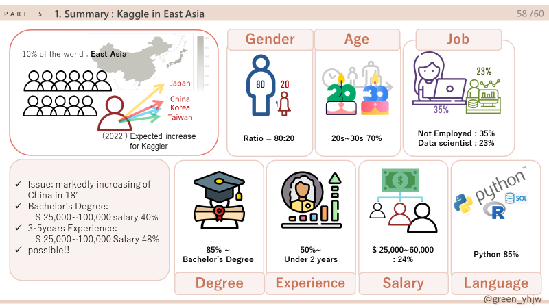
1.3 Summary
used data
We used all the data for five years. (2017~2021)
used Language and Library
- Numpy
- Metplotlib
- seaborn
- Plotly
- plotly.express : An interface where you can draw a graph easily and quickly.
- plotly.graph_objects : You can customize it in the way you want because you can do more detailed work than express.
- plotly.figure_factory : Used before express existed and remains in the module for compatibility with previous versions
- plotly.subplots : A module that displays multiple graphs in one figure.
- plotly.offline : Save locally and create HTML that opens in a web browser and make it standalone
Grouping data sections
- East Asia and World
- East Asia : [‘China’,’Taiwan’, ‘South Korea’, ‘Japan’]
- World : all data
- Gender
- [Male, Female, Others]
- Job
- Data_Analyst =[‘Data Analyst’,’Data Miner,Information technology’,’Data Miner’,
'Predictive Modeler','Information technology, networking, or system administration', 'A business discipline (accounting, economics, finance, etc.)', 'Business Analyst', Humanities', 'Statistician', 'Mathematics or statistics', 'Medical or life sciences (biology, chemistry, medicine, etc.)', Physics or astronomy', 'Social sciences (anthropology, psychology, sociology, etc.)', 'Environmental science or geology', 'Humanities (history, literature, philosophy, etc.)'] - Data_Scientist =[‘Data Scientist’, ‘Research Scientist’, ‘Researcher’,’Machine Learning Engineer’, ‘Scientist/Researcher’]
- Developer=[‘Developer Relations/Advocacy’,’Data Engineer’,’Engineer’,’Engineering (non-computer focused)’,
‘Programmer’,’Software Engineer’, ‘Computer Scientist’,’Computer science (software engineering, etc.)’, ‘Fine arts or performing arts’,’Product Manager’, ‘Software Developer/Software Engineer’, ‘Product/Project Manager’,’Program/Project Manager’,’DBA/Database Engineer’] - Not_Employed =[‘Currently not employed’, ‘Not employed’, ‘Student’]
- Others = [‘I never declared a major’, ‘Other’]
- Data_Analyst =[‘Data Analyst’,’Data Miner,Information technology’,’Data Miner’,
- Age
- [18-21, 20s, 30s, 40s, 50s, 60s<]
- Degree
- [‘
college’, ‘Bachelor’s degree’,’Master’s degree’, ‘Doctoral degree‘, ‘etc’]
- [‘
- Experience
- [<1, 1-3, 3-5, 5-10, 10+]
- Salary
- [<999, 1,000-20,000, 20,000-59,999, 60,000-99,999, 100,000-199,999, 200,000~]
2. data Import and pre-treatments
1 | import numpy as np |
1 | df17= pd.read_csv("/kaggle/input/kaggle-survey-2017/multipleChoiceResponses.csv", encoding="ISO-8859-1") |
3. plots and description
1 |
|
3.1 Kaggle’s transformation (World/East Asia)
3.1.1 user transformation
Number of respondents
(bar, scatter plot : number of respondents to World and East Asia,
Map plot : number of respondents to East Asia)
World and East Asia: The same trend.
East Asia: 15% of the total continent and 20.3% of the population (16/78.7: Ea/Wo)
2018 Issue: Significant increase in respondents->Hypothesis: Due to the rapid increase in China.
2018 Outliers Considering: 2022 Kaggle survey Respondents: Increased in both World and East Asia
I wish our team the honor of becoming a respondent to the Kaggle survey in 2022….
1 | fig = go.Figure() |
18’ :
User change between United States and India.
China’s markedly increase in 2018
- There is no Taiwan, but only China has increased. : East Asian political situation Issue can be suspected.
1 | A18 = ( |
Total population:
1.4 billion (85%) in China, 130 million in Japan, 0.5 billion in Korea, and 0.2 billion in Taiwan.
- China: The number of respondents is smaller than the population.
- Japan: Starting in 2019, overtaking China
- Taiwan : 2018 data 0 =? Diplomatic issues? The growth trend is weak.
- Korea : Respondents at a similar level to Japan’s population.
- East Asia: The number of respondents will increase further.
1 | #data preprocessing |
1 | fig = go.Figure(data=[ |
3.1.2 Gender transformation
World: The proportion of female respondents increases (still below 20%)
The number of respondents is increasing in all genders.
Our team is also a team with high female members and wants to contribute as a respondent in 2022.
1 | #data preprocessing |
- Male (1004->2037 : 2017->2021) double increase

- Female 183->327 : 2017->2021 increased 1.8 times

- Others (8->64 : 2017->2021) 8x increase
[Compare the high and low points]
- Male (1004->2037 : 2017->2021) double increase
- Female 183->327 : 2017->2021 increased 1.8 times
- Others (8->64 : 2017->2021) 8x increase
It can be seen that the number of female respondents and the ratio of male respondents hardly change, which is a difference compared to World data.
It can be seen that the degree of gender freedom in East Asia has increased relatively.
Compared to World data, it can be seen that in 2021 (1.87: 2.6= Wo: Ea), compared to 2017 (1.96: 0.7 = Ea), which was relatively conservative.
1 | #data preprocessing |
3.1.3 Job transformation
21' World Vs East Asia Age Ratio: Bar plot
Not Employed : More than 30% in both East Asia and the world, the highest.
Because “Students” is included.
Data Scientist : High percentage in the world and East Asia.
Relatively low proportion in East Asia.
= Absolute lack of numbers
We would like to move forward by selecting a **data scientist** with insufficient numbers in East Asia.
1 | #data preprocessing |
World Job Ratio: Heat Map
The trend of increasing each job except Others.
Data Scientist has a high proportion, and the trend is to increase further in 2022.
East Asia Job Ratio: Heat Map
East Asia : Increasing the ratio of data scientist.1 | #data preprocessing |
3.1.4 Age transformation
> Age change in World and East Asia by year: Stacked scatter plot
- In the case of Age data, there is no 2017 data.
- 70% of the World respondents said 20s to 30s.
- 70% of East Asia respondents said 20s to 30s.
- The number of respondents increases, but the ratio seems to have stabilized.
1 | #data preprocessing |
17'East Asia Age Ratio: Heat Map
- East Asia : 50% or more. Those in their 20s and 30s.
- Korea: Those in their 20s are the highest.
The number of respondents in their 50s and older is also large. - Taiwan : The number of respondents in their 30s and older is relatively small.
- China: 70% or more of respondents in their 30s or younger.
Related to life expectancy? - Japan: Like an aging country, all ages are evenly distributed.
Even if you’re older, there are many respondents to Kaggle.
1 | #data processing |
17’East Asia’s age ratio: Box plot
2017: Data is not a section but an individual number.
If you divide the interval, you can add it to the previous graph.
It was data that I could draw a bar plot, so I drew it.
You can see a 100-year-old in China, but they don’t remove missing values on purpose.
1 | # 연도별 나이 |
3.1.5 Degree transformation
World job ratio in each country: pie plot
- World: 90% or higher Bachelor’s degree
- East Asia: 85% bachelor’s degree or higher
1 | #data preprocessing |
Percentage of East Asia degrees by year: sunburst plot
The highest percentage of respondents with master’s degrees per year
1 | #data preprocessing |
Plus we could see the advantages of Plotly in this graph.
Matplotlib draws a static graph, but Plotly can dynamically click and move, and it supports zooming out, zooming in, and downloading graphs.
Because all of our graphs are made of plotly, the viewer can represent or remove items in the graph if desired.
With a click
East Asia Degree Ratio: Bar plot
40% of master’s degrees or higher, and respondents have a high educational background.
- China and Japan have similar trends to East Asia and the World.
The number of people itself is large, so a representative trend seems to appear here.
However, it is noteworthy that the two countries have the same tendency.
Korea: It is the only country among the four countries with a high degree of education below Ph.D., bachelor’s degree, and junior college. Only masters are low.
(Polarization of education?)Taiwan: 1st place in master’s ratio (55%), 2nd place in Ph.D. or higher (13.8%).
= The highest level of education.
1 | #data preprocessing |
3.1.6 Experience transformation
Trends in World & East Asia Career: Stacked Scatter plot
- < 2 years: 50% of the total.- 3-5 years: Decrease in the world, maintain East Asia ratio
- 2021 'etc data' disappeared.
1 | #Exp data 전처리 |
1 | #data preprocessing |
3.1.7 Salary transformation
World & East Asia Annual salary: Bar-H plot
- $ 200,000 ~ : World (2.9%) is more than 50% compared to East Asia (1.3%)
- $ ~250,000 : World (59.2%) is less than East Asia (50.3%)
= East Asia’s annual salary gap between rich and poor is less. - $ 25,000~60,000: The highest section in East Asia at 24%.
= The annual salary section that we aim for.
1 | #data preprocessing |
World experience and annual salary: Heat Map
Relatively **positive correlation.**
Even with 5-10 years of experience, more than 45% has an annual salary of less than $20,000
With more than 10 years of experience, more than 30% receive an annual salary of $100,000.
1 | #data preprocessing |
World & East Asia Degree/Annual salary: Heat Map
- \$ ~20,000 : Regardless of degree, about 40% of the annual salary is $ 20,000 or less.
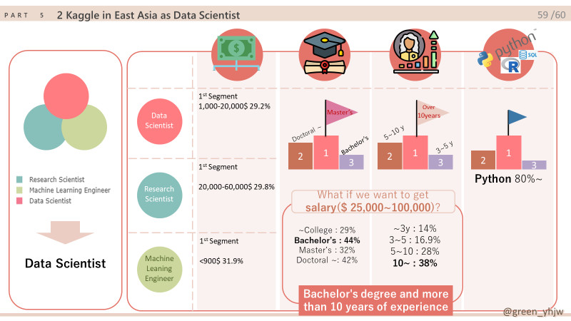
Guess it’s the ratio that comes from a student. - $ 25,000-100,000 : Earned more than 40% with a bachelor’s degree alone in East Asia
(World: less than 20%) - $ 200,000~ : Even with a doctorate or higher, it is difficult to obtain it from East Asia.
1 | #data preprocessing |
3.1.8 Language transformation
World & East Asia Programming Language: Bar plot
- Python: 80% of the world and 85% of East Asia use it.We've been working on the project as python, so I hope we can continue to learn python and become experienced Data Scientists!
1 | #data preprocessing |
1 | #data prprocessing |
3.2 Position of Data Scientist in East Asia
1 | # data preprocessing |
3.2.1 Salary
1 | df21_Ea_DS_= df21_Ea_DS.loc[:,['Q5','Q25']].reset_index().rename(columns={'Q5':'Data_Scientist', 'Q25':'Salary'}).fillna('etc') |
3.2.2 Salary-Experience
1 | df21Ea_DS_ExSal = df21_Ea_DS.loc[:,['Q6','Q25']].reset_index().rename(columns={'Q25':'Salary', 'Q6':'Exp'}).fillna('etc') |
3.2.3 Degree
1 | df21_Ea_degree = df21_Ea_DS['Q4'].value_counts().to_frame() |
3.2.4 Salary-Degree
1 | df21Ea_DS_EduSal= df21_Ea_DS.loc[:, ['Q4', 'Q25']].rename(columns={'Q4':'Edu', 'Q25':'Salary'}) |
3.2.5 Language
1 | #data preprocessing |
1 | ds_pc=(df21_Ea_DS.loc[:, ['Q5','Q25','Q6','Q4','Q8']] |
4. Ref.
Ref.
동아시아 지역 https://ko.wikipedia.org/wiki/%EB%8F%99%EC%95%84%EC%8B%9C%EC%95%84
동아시아 인구 https://ko.wikipedia.org/wiki/%EC%95%84%EC%8B%9C%EC%95%84%EC%9D%98_%EC%9D%B8%EA%B5%AC
세계 인구 https://ko.wikipedia.org/wiki/%EC%84%B8%EA%B3%84_%EC%9D%B8%EA%B5%AC
https://ko.wikipedia.org/wiki/%EC%9D%B8%EA%B0%84_%EA%B0%9C%EB%B0%9C_%EC%A7%80%EC%88%98#2020%EB%85%84동아시아 인간개발지수 https://namu.wiki/w/%EB%8F%99%EC%95%84%EC%8B%9C%EC%95%84
Data Scientist란 https://dataprofessional.tistory.com/126
https://terms.naver.com/entry.naver?docId=1691563&cid=42171&categoryId=42183Python이란 https://ko.wikipedia.org/wiki/%ED%8C%8C%EC%9D%B4%EC%8D%AC
Kaggle competition Ref. https://www.kaggle.com/miguelfzzz/the-typical-kaggle-data-scientist-in-2021
https://www.kaggle.com/desalegngeb/how-popular-is-kaggle-in-africa
- flaricon: Icons made by Freepik from www.flaticon.com
5. close
안녕하세요 한국에 사는 YH입니다.
python을 배운지 한달이 채 안되서 명이 한 팀이 되어 이번 대회에 참가 하게 되었습니다.
많이 부족하지만 여기까지 읽어 주셔서 감사합니다.
아직은 너무너무 부족한 제출물 이지만, 앞으로 열심히 해서 케글 대회에서 1등하는 그 날까지 지켜봐 주세요 ^^!
혹시 코멘트로 다 전하지 못하셨던 말이 있으시다면, 저의 github blog에 방문하여 도움을 주세요!
별거 없지만 놀러오세요 ;-)
Hello, I’m YH and I live in Korea.
Less than a month after learning python, people became a team and participated in this competition.
It’s not enough, but thank you for reading it up to here.
It’s still not enough, but please watch until the day we win first place at the Kaggle competition ^^!
If there’s anything you haven’t said in the comments, please visit my github blog and help me!
It’s nothing special, but come and play. ;-)
Newbie as a data scientist in East Asia! (kaggle Competition)
https://yoonhwa-p.github.io/2021/11/28/kgg/KaggleCompetition_ver33byYH_Finall/
install_url to use ShareThis. Please set it in _config.yml.