visualization by python

Visualization _python으로

[1103 학습]
시각화 연습 및 작성 코드 깃헙 블로그 및 깃헙에 올리기, 개인별로 공유

  • 시각화 올릴 때, 전체 코드 올리지 마시고,
    나눠서 올리세요. 설명 글 추가하시고여~ (예시 하단)

    산점도: 산점도란 무엇인가? 언제 쓰는가? 코드 작성 및 간단 설명
    박스플롯: 박스플롯이란 무엇인가? 언제 쓰는가? 코드 작성 및 간단 설명

오후 1시까지 1차로 한번 올려서 개인별로 공유해주세요. 홧팅요

Intro

python에서 visualiztion 하기 위해서는 많은 방법이 있다.

data Analist들은 시각화를 위해 많은 tool을 사용 하는데 우리는 SeabornMatplotlib을 이용하여 시각화를 할 예정이다.


코드 기반(python)의 data visualiztion의 장점

  • 여러 그래프 동시 작성 가능
  • 기존의 코드 재활용성
  • 데이터 그기의 제한이 없음 (RAM등의 제약조건 없을때)

Matplotlib 는 이미지 데이터와 정형 데이터(정적 그래프)를 시각화 할 수 있는데 나와 같은 비전공자들에게 시각화 문법이 조금 어렵다고 한다. 하지만 pandas data frame에서 쉽게 시각화 구현 하며, 통계(회귀선) 그래프 등을 쉽게 구현 할 수 있기 때문에 이를 배워야 한다.

seaborn의 경우 그래프가 예쁘게 나오지 않지만 비교적 간단한 코드로 시각화를 할 수 있다. 하지만, 세부 옵션을 수정 하고 싶다면 Matplotlib를 알아야 한다. 이는 내부 원리를 파악 할 수 없기 때문에 내가 감당하기 힘들다.

때문에 지금 단계에서는 Matplotlib과 seaborn의 장점을 적절하게 섞어서 시각화를 진행 해 보자.


아래와 같은 Tutorial을 진행 하면 세부 옵션을 조정 하기 쉽다고 한다.
https://matplotlib.org/stable/tutorials/index.html

matplotlib

matplotlib를 이용하여 visualiztion을 해 보자.

제일 먼저 해 주어야 할 일은 Import하여 matplotlib를 불러오고 이를 plt등의 객체에 저장 해 주는 것이다.

1
2
3
4
5
6
7
8
9
import matplotlib.pyplot as plt

dates = [
'2021-01-01', '2021-01-02', '2021-01-03', '2021-01-04', '2021-01-05',
'2021-01-06', '2021-01-07', '2021-01-08', '2021-01-09', '2021-01-10'
]
min_temperature = [20.7, 17.9, 18.8, 14.6, 15.8, 15.8, 15.8, 17.4, 21.8, 20.0]
max_temperature = [34.7, 28.9, 31.8, 25.6, 28.8, 21.8, 22.8, 28.4, 30.8, 32.0]

위의 data는 강사님의 data를 가져 온 것이다.

data를 시각화 자료로 만들어 보자,

1
2
3
4
5
fig, axes = plt.subplots(nrows=1, ncols=1, figsize=(10,6))
axes.plot(dates, min_temperature, label = 'Min Temperature')
axes.plot(dates, max_temperature, label = 'Max Temperature')
axes.legend()
plt.show()

graph

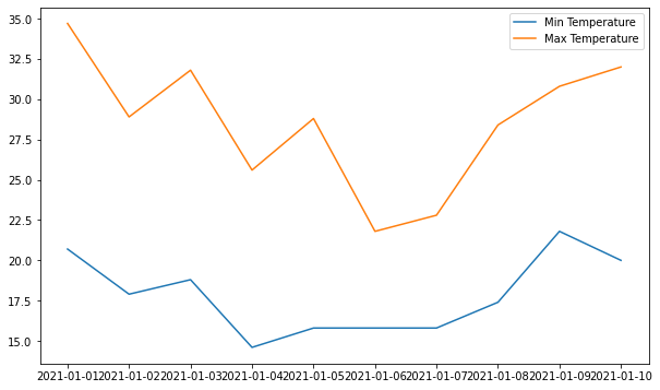
위의 표는 legend가 있고, 날짜별로 Min Temp와 Max Temp가 있는 그래프 이다.

먼저 fig, ax = plt.subplots()를 이용하여 표를 생성 한다.

이때 figure에대한 정보를 함께 생성 할 수 있는데, (nrows=1, ncols=1, figsize=(10,6)) 가 의미하는 것은 (행의 갯수 =1, 열의 갯수=1, fig size는 10X6)이다.

ax를 통하여 plot 형태의 그래프를 그리는데, (x축, y축 , label = “[name]”)의 형태로 plot을 추가 해 준다.
이때 Legend 를 생성 하고 싶다면, ax.legend()함수로 추가 해 줄 수 있다.

마지막으로 plt.show() 를 사용하여 마무리 해 준다.

물론 마지막 코드를 넣지 않아도 보여 주지만, 넣어주는 것이 인지상정이라고 한다.

1
2
3
print(fig)
print(axes)

Figure(720x432)
AxesSubplot(0.125,0.125;0.775x0.755)

위의 표인 fig의 정보를 알 수 있게 print 함수로 뽑아 봤는데 이건 무슨 말 인지 잘 모르겠다.

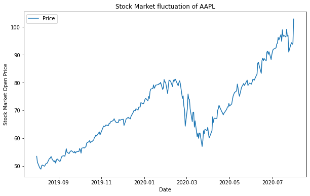
matplotlib로 선 그래프 그리기

아직 data를 어디에서 받을 수 있는지 잘 모르기 때문에 강사님이 다운받은 표를 그대로 가져와 보자

참조: https://pypi.org/project/fix-yahoo-finance/

1
!pip install yfinance --upgrade --no-cache-dir
Collecting yfinance
  Downloading yfinance-0.1.64.tar.gz (26 kB)
Requirement already satisfied: pandas>=0.24 in /usr/local/lib/python3.7/dist-packages (from yfinance) (1.1.5)
Requirement already satisfied: numpy>=1.15 in /usr/local/lib/python3.7/dist-packages (from yfinance) (1.19.5)
Requirement already satisfied: requests>=2.20 in /usr/local/lib/python3.7/dist-packages (from yfinance) (2.23.0)
Requirement already satisfied: multitasking>=0.0.7 in /usr/local/lib/python3.7/dist-packages (from yfinance) (0.0.9)
Collecting lxml>=4.5.1
  Downloading lxml-4.6.4-cp37-cp37m-manylinux_2_17_x86_64.manylinux2014_x86_64.manylinux_2_24_x86_64.whl (6.3 MB)
     |████████████████████████████████| 6.3 MB 7.7 MB/s 
[?25hRequirement already satisfied: python-dateutil>=2.7.3 in /usr/local/lib/python3.7/dist-packages (from pandas>=0.24->yfinance) (2.8.2)
Requirement already satisfied: pytz>=2017.2 in /usr/local/lib/python3.7/dist-packages (from pandas>=0.24->yfinance) (2018.9)
Requirement already satisfied: six>=1.5 in /usr/local/lib/python3.7/dist-packages (from python-dateutil>=2.7.3->pandas>=0.24->yfinance) (1.15.0)
Requirement already satisfied: urllib3!=1.25.0,!=1.25.1,<1.26,>=1.21.1 in /usr/local/lib/python3.7/dist-packages (from requests>=2.20->yfinance) (1.24.3)
Requirement already satisfied: chardet<4,>=3.0.2 in /usr/local/lib/python3.7/dist-packages (from requests>=2.20->yfinance) (3.0.4)
Requirement already satisfied: idna<3,>=2.5 in /usr/local/lib/python3.7/dist-packages (from requests>=2.20->yfinance) (2.10)
Requirement already satisfied: certifi>=2017.4.17 in /usr/local/lib/python3.7/dist-packages (from requests>=2.20->yfinance) (2021.5.30)
Building wheels for collected packages: yfinance
  Building wheel for yfinance (setup.py) ... [?25l[?25hdone
  Created wheel for yfinance: filename=yfinance-0.1.64-py2.py3-none-any.whl size=24109 sha256=25a6e16cba240e66cb4999d0947a231b790b2b96766767434407e09149ec9302
  Stored in directory: /tmp/pip-ephem-wheel-cache-a8wml444/wheels/86/fe/9b/a4d3d78796b699e37065e5b6c27b75cff448ddb8b24943c288
Successfully built yfinance
Installing collected packages: lxml, yfinance
  Attempting uninstall: lxml
    Found existing installation: lxml 4.2.6
    Uninstalling lxml-4.2.6:
      Successfully uninstalled lxml-4.2.6
Successfully installed lxml-4.6.4 yfinance-0.1.64
1
2
3
4
5
6
import yfinance as yf

data= yf.download('AAPL', '2019-08-01', '2021-08-01')
data.info()
print(yf)

[*********************100%***********************]  1 of 1 completed
<class 'pandas.core.frame.DataFrame'>
DatetimeIndex: 504 entries, 2019-08-01 to 2021-07-30
Data columns (total 6 columns):
 #   Column     Non-Null Count  Dtype  
---  ------     --------------  -----  
 0   Open       504 non-null    float64
 1   High       504 non-null    float64
 2   Low        504 non-null    float64
 3   Close      504 non-null    float64
 4   Adj Close  504 non-null    float64
 5   Volume     504 non-null    int64  
dtypes: float64(5), int64(1)
memory usage: 27.6 KB
<module 'yfinance' from '/usr/local/lib/python3.7/dist-packages/yfinance/__init__.py'>

info() 함수를 통해 column정보와 data의 갯수, data의 type까지 알 수 있다.
date time index에 구간이 내가 정한데로 나와 있는 것도 볼 수 있다.

1
2
ts = data['Open']
print(ts.head())
Date
2019-08-01    53.474998
2019-08-02    51.382500
2019-08-05    49.497501
2019-08-06    49.077499
2019-08-07    48.852501
Name: Open, dtype: float64

ts 객체에 Open data를 담고 .head() 함수로 상위 5개의 항목을 가져와 본다.

혹시,
Pandas 에대하여 더 정리된 것을 알고 싶다면, 링크를 통해 확인 할 수 있다.

Pyplot API

아래의 예는 Pyplot API 방법을 이용하여, 한개씩 data를 넣어 준 형태 이다. 이는 객체지향으로 만들었다고 하기 어렵지만, 가능은 하다.

1
2
3
4
5
6
7
8
9
10
11
12
13
# import fix_yahoo_finance as yf
import yfinance as yf
import matplotlib.pyplot as plt

data = yf.download('AAPL', '2019-08-01', '2020-08-01')
ts = data['Open']
plt.figure(figsize=(10,6))
plt.plot(ts)
plt.legend(labels=['Price'], loc='best')
plt.title('Stock Market fluctuation of AAPL')
plt.xlabel('Date')
plt.ylabel('Stock Market Open Price')
plt.show()
[*********************100%***********************]  1 of 1 completed

graph

Pyplot API 객체지향

1
2
3
4
5
from matplotlib.backends.backend_agg
import FigureCanvasAgg as FigureCanvas
from matplotlib.figure import Figure
import matplotlib.pyplot as plt

객체지향을 위해 import를 해 준다.

1
2
3
4
5
6
7
8
9
10
11
fig = Figure()

import numpy as np
np.random.seed(6)
x = np.random.randn(20000)

ax = fig.add_subplot(111)
ax.hist(x, 100)
ax.set_title('Artist Layer Histogram')
# fig.savefig('Matplotlib_histogram.png')
plt.show()

166
167
168
169
170
171
172
173
174
175
176
177
178
179
180
181
182
183
184
185
186
187
188
189
190
191
192
193
194
195
196
197
198
199
200
201
202
203
204
205
206
207
208
209
210
211
212
213
214
215
216
217
218
219
220
[{'efcvTrfl': '18',
'endUnitCode': '103 ',
'endUnitNm': '수원신갈',
'iEndUnitCode': None,
'iStartEndStdTypeCode': None,
'iStartUnitCode': None,
'numOfRows': None,
'pageNo': None,
'startEndStdTypeCode': '2',
'startEndStdTypeNm': '도착기준통행시간',
'startUnitCode': '101 ',
'startUnitNm': '서울',
'stdDate': '20220103',
'stdTime': '00:25',
'sumTmUnitTypeCode': None,
'tcsCarTypeCode': '1',
'tcsCarTypeDivCode': '1',
'tcsCarTypeDivName': '소형차',
'tcsCarTypeName': '1종',
'timeAvg': '7.466666666666667',
'timeMax': '9.216',
'timeMin': '5.800'},
{'efcvTrfl': '53',
'endUnitCode': '103 ',
'endUnitNm': '수원신갈',
'iEndUnitCode': None,
'iStartEndStdTypeCode': None,
'iStartUnitCode': None,
'numOfRows': None,
'pageNo': None,
'startEndStdTypeCode': '2',
'startEndStdTypeNm': '도착기준통행시간',
'startUnitCode': '101 ',
'startUnitNm': '서울',
'stdDate': '20220103',
'stdTime': '00:30',
'sumTmUnitTypeCode': None,
'tcsCarTypeCode': '1',
'tcsCarTypeDivCode': '1',
'tcsCarTypeDivName': '소형차',
'tcsCarTypeName': '1종',
'timeAvg': '7.466666666666667',
'timeMax': '9.283',
'timeMin': '5.783'},
{'efcvTrfl': '14',
'endUnitCode': '103 ',
'endUnitNm': '수원신갈',
'iEndUnitCode': None,
'iStartEndStdTypeCode': None,
'iStartUnitCode': None,
'numOfRows': None,
'pageNo': None,
'startEndStdTypeCode': '2',
'startEndStdTypeNm': '도착기준통행시간',
'startUnitCode': '101 ',
'startUnitNm': '서울',
'stdDate': '20220103',
'stdTime': '00:35',
'sumTmUnitTypeCode': None,
'tcsCarTypeCode': '1',
'tcsCarTypeDivCode': '1',
'tcsCarTypeDivName': '소형차',
'tcsCarTypeName': '1종',
'timeAvg': '7.416666666666667',
'timeMax': '8.400',
'timeMin': '6.050'},
{'efcvTrfl': '15',
'endUnitCode': '103 ',
'endUnitNm': '수원신갈',
'iEndUnitCode': None,
'iStartEndStdTypeCode': None,
'iStartUnitCode': None,
'numOfRows': None,
'pageNo': None,
'startEndStdTypeCode': '2',
'startEndStdTypeNm': '도착기준통행시간',
'startUnitCode': '101 ',
'startUnitNm': '서울',
'stdDate': '20220103',
'stdTime': '00:40',
'sumTmUnitTypeCode': None,
'tcsCarTypeCode': '1',
'tcsCarTypeDivCode': '1',
'tcsCarTypeDivName': '소형차',
'tcsCarTypeName': '1종',
'timeAvg': '7.516666666666667',
'timeMax': '9.283',
'timeMin': '5.966'},
{'efcvTrfl': '41',
'endUnitCode': '103 ',
'endUnitNm': '수원신갈',
'iEndUnitCode': None,
'iStartEndStdTypeCode': None,
'iStartUnitCode': None,
'numOfRows': None,
'pageNo': None,
'startEndStdTypeCode': '2',
'startEndStdTypeNm': '도착기준통행시간',
'startUnitCode': '101 ',
'startUnitNm': '서울',
'stdDate': '20220103',
'stdTime': '00:45',
'sumTmUnitTypeCode': None,
'tcsCarTypeCode': '1',
'tcsCarTypeDivCode': '1',
'tcsCarTypeDivName': '소형차',
'tcsCarTypeName': '1종',
'timeAvg': '7.5',
'timeMax': '8.800',
'timeMin': '5.750'},
{'efcvTrfl': '11',
'endUnitCode': '103 ',
'endUnitNm': '수원신갈',
'iEndUnitCode': None,
'iStartEndStdTypeCode': None,
'iStartUnitCode': None,
'numOfRows': None,
'pageNo': None,
'startEndStdTypeCode': '2',
'startEndStdTypeNm': '도착기준통행시간',
'startUnitCode': '101 ',
'startUnitNm': '서울',
'stdDate': '20220103',
'stdTime': '00:50',
'sumTmUnitTypeCode': None,
'tcsCarTypeCode': '1',
'tcsCarTypeDivCode': '1',
'tcsCarTypeDivName': '소형차',
'tcsCarTypeName': '1종',
'timeAvg': '7.416666666666667',
'timeMax': '8.800',
'timeMin': '5.766'},
{'efcvTrfl': '8',
'endUnitCode': '103 ',
'endUnitNm': '수원신갈',
'iEndUnitCode': None,
'iStartEndStdTypeCode': None,
'iStartUnitCode': None,
'numOfRows': None,
'pageNo': None,
'startEndStdTypeCode': '2',
'startEndStdTypeNm': '도착기준통행시간',
'startUnitCode': '101 ',
'startUnitNm': '서울',
'stdDate': '20220103',
'stdTime': '00:55',
'sumTmUnitTypeCode': None,
'tcsCarTypeCode': '1',
'tcsCarTypeDivCode': '1',
'tcsCarTypeDivName': '소형차',
'tcsCarTypeName': '1종',
'timeAvg': '7.433333333333334',
'timeMax': '8.350',
'timeMin': '5.750'},
{'efcvTrfl': '87',
'endUnitCode': '103 ',
'endUnitNm': '수원신갈',
'iEndUnitCode': None,
'iStartEndStdTypeCode': None,
'iStartUnitCode': None,
'numOfRows': None,
'pageNo': None,
'startEndStdTypeCode': '2',
'startEndStdTypeNm': '도착기준통행시간',
'startUnitCode': '101 ',
'startUnitNm': '서울',
'stdDate': '20220103',
'stdTime': '01 ',
'sumTmUnitTypeCode': None,
'tcsCarTypeCode': '1',
'tcsCarTypeDivCode': '1',
'tcsCarTypeDivName': '소형차',
'tcsCarTypeName': '1종',
'timeAvg': '7.55',
'timeMax': '10.183',
'timeMin': '5.750'},
{'efcvTrfl': '30',
'endUnitCode': '103 ',
'endUnitNm': '수원신갈',
'iEndUnitCode': None,
'iStartEndStdTypeCode': None,
'iStartUnitCode': None,
'numOfRows': None,
'pageNo': None,
'startEndStdTypeCode': '2',
'startEndStdTypeNm': '도착기준통행시간',
'startUnitCode': '101 ',
'startUnitNm': '서울',
'stdDate': '20220103',
'stdTime': '01:00',
'sumTmUnitTypeCode': None,
'tcsCarTypeCode': '1',
'tcsCarTypeDivCode': '1',
'tcsCarTypeDivName': '소형차',
'tcsCarTypeName': '1종',
'timeAvg': '7.625',
'timeMax': '10.183',
'timeMin': '6.600'},
{'efcvTrfl': '3',
'endUnitCode': '103 ',
'endUnitNm': '수원신갈',
'iEndUnitCode': None,
'iStartEndStdTypeCode': None,
'iStartUnitCode': None,
'numOfRows': None,
'pageNo': None,
'startEndStdTypeCode': '2',
'startEndStdTypeNm': '도착기준통행시간',
'startUnitCode': '101 ',
'startUnitNm': '서울',
'stdDate': '20220103',
'stdTime': '01:05',
'sumTmUnitTypeCode': None,
'tcsCarTypeCode': '1',
'tcsCarTypeDivCode': '1',
'tcsCarTypeDivName': '소형차',
'tcsCarTypeName': '1종',
'timeAvg': '7.683333333333334',
'timeMax': '8.250',
'timeMin': '7.500'}]

04.4 csv file로 출력

1
2
3
4
5
6
7
8
9
10
11
import pandas as pd
dt = []
for car in cars:
dic_df = {}
dic_df["data"] = car["stdDate"]
dic_df["time"] = car["stdTime"]
dic_df["destination"] = car["endUnitNm"]
dt.append(dic_df)

pd.DataFrame(dt).to_csv("temp.csv",index = False, encoding="euc-kr")

Encoding의 경우 해당 json file의 documents를 봐야함.

google과 같은 기업에서 API를 받아와서 사용 하는 것도 가능 하므로
앞으로 이 기술은 무궁무진한 발전 가능성이 있을 것으로 보임 ^^

DTS: ML_Grid search(Hyper Parameter)

§ 이전 posting

PipeLine

Learning curve


ML pipeLine 검증 곡선 그리기

  • ML 그리드 서치

    • grid search를 이용한 파이프라인(pipeLine) 설계및
      하이퍼 파라미터 튜닝(hyper parameter)
    • 그리드 서치와 랜덤 서치가 있다.
      • 랜덤 서치로 먼저 뽑아 낸 후 그리드 서치를 이용하여 안정적으로 서치 !
  • 나도 공부 하기 싫으닌까 그냥
    이 하는거 따라 쓰고 싶다.

남 : Kaggle competition


1
2
3
4
5
6
7
8
9
10
11
12
13
14
15
16
17
18
19
20
21
22
23
24
25
26
27
28
29
30
31
32
33
34
35
36
37
38
import pandas as pd 
from sklearn.preprocessing import LabelEncoder
from sklearn.model_selection import train_test_split
import numpy as np
from sklearn.model_selection import StratifiedKFold
from sklearn.linear_model import LogisticRegression
from sklearn.pipeline import make_pipeline
from sklearn.preprocessing import StandardScaler
from sklearn.decomposition import PCA
import matplotlib.pyplot as plt
from sklearn.model_selection import learning_curve
from sklearn.model_selection import validation_curve
from sklearn.tree import DecisionTreeClassifier
from sklearn.model_selection import GridSearchCV
from sklearn.svm import SVC

data_url = 'https://archive.ics.uci.edu/ml/machine-learning-databases/breast-cancer-wisconsin/wdbc.data'
column_name = ['id', 'diagnosis', 'radius_mean', 'texture_mean', 'perimeter_mean', 'area_mean', 'smoothness_mean', 'compactness_mean', 'concavity_mean',
'concave points_mean', 'symmetry_mean', 'fractal_dimension_mean', 'radius_se', 'texture_se', 'perimeter_se', 'area_se', 'smoothness_se',
'compactness_se', 'concavity_se', 'concave points_se', 'symmetry_se', 'fractal_dimension_se', 'radius_worst', 'texture_worst', 'perimeter_worst',
'area_worst', 'smoothness_worst', 'compactness_worst', 'concavity_worst', 'concave points_worst', 'symmetry_worst', 'fractal_dimension_worst']

df = pd.read_csv(data_url, names=column_name)

X = df.loc[:, "radius_mean":].values
y = df.loc[:, "diagnosis"].values

le = LabelEncoder()
y = le.fit_transform(y)

X_train, X_test, y_train, y_test = train_test_split(X, y, test_size = 0.20,
# stratify = y,
random_state=1)
kfold = StratifiedKFold(n_splits = 10, random_state=1, shuffle=True)

pipe_tree = make_pipeline(StandardScaler(),
PCA(n_components=2),
DecisionTreeClassifier(random_state=1))
1
2
3
4
5
6
7
8
9
10
11
12
13
14
15
16
17
18
19
20
21
# 이 Line이 핵쉼 !!

# estimator.get_params().keys()
# pipe_tree.get_params().keys() ---> 이렇게 씀.

print(pipe_tree.get_params().keys())
param_grid = [{"decisiontreeclassifier__max_depth": [1, 2, 3, 4, 5, 6, 7, None]}]

gs = GridSearchCV(estimator = pipe_tree,
param_grid = param_grid,
scoring="accuracy",
cv = kfold)

gs = gs.fit(X_train, y_train)
print(gs.best_score_)
print(gs.best_params_)

clf = gs.best_estimator_
# 자동으로 제일 좋은 것을 뽑아서 알려줌.
clf.fit(X_train, y_train)
print("테스트 정확도:", clf.score(X_test, y_test))

dict_keys([‘memory’, ‘steps’, ‘verbose’, ‘standardscaler’, ‘pca’, ‘decisiontreeclassifier’, ‘standardscaler__copy’, ‘standardscaler__with_mean’, ‘standardscaler__with_std’, ‘pca__copy’, ‘pca__iterated_power’, ‘pca__n_components’, ‘pca__random_state’, ‘pca__svd_solver’, ‘pca__tol’, ‘pca__whiten’, ‘decisiontreeclassifier__ccp_alpha’, ‘decisiontreeclassifier__class_weight’, ‘decisiontreeclassifier__criterion’, ‘decisiontreeclassifier__max_depth’, ‘decisiontreeclassifier__max_features’, ‘decisiontreeclassifier__max_leaf_nodes’, ‘decisiontreeclassifier__min_impurity_decrease’, ‘decisiontreeclassifier__min_samples_leaf’, ‘decisiontreeclassifier__min_samples_split’, ‘decisiontreeclassifier__min_weight_fraction_leaf’, ‘decisiontreeclassifier__random_state’, ‘decisiontreeclassifier__splitter’])
0.927536231884058
{‘decisiontreeclassifier__max_depth’: 7}
테스트 정확도: 0.9210526315789473

svc를 이용한 hyperparameter tuenning

1
2
3
4
5
6
7
8
9
10
11
12
13
14
15
16
17
18
19
20
21
22
23
24
25
26
27
28
29
30
31
32
33
34
35
36
37
38
39
40
41
42
43
44
45
46
47
48
49
50
51
52
53
54
55
import pandas as pd 
from sklearn.preprocessing import LabelEncoder
from sklearn.model_selection import train_test_split
import numpy as np
from sklearn.model_selection import StratifiedKFold
from sklearn.linear_model import LogisticRegression
from sklearn.pipeline import make_pipeline
from sklearn.preprocessing import StandardScaler
from sklearn.decomposition import PCA
import matplotlib.pyplot as plt
from sklearn.model_selection import learning_curve
from sklearn.model_selection import validation_curve
from lightgbm import LGBMClassifier
from sklearn.model_selection import GridSearchCV
from sklearn.svm import SVC

data_url = 'https://archive.ics.uci.edu/ml/machine-learning-databases/breast-cancer-wisconsin/wdbc.data'
column_name = ['id', 'diagnosis', 'radius_mean', 'texture_mean', 'perimeter_mean', 'area_mean', 'smoothness_mean', 'compactness_mean', 'concavity_mean',
'concave points_mean', 'symmetry_mean', 'fractal_dimension_mean', 'radius_se', 'texture_se', 'perimeter_se', 'area_se', 'smoothness_se',
'compactness_se', 'concavity_se', 'concave points_se', 'symmetry_se', 'fractal_dimension_se', 'radius_worst', 'texture_worst', 'perimeter_worst',
'area_worst', 'smoothness_worst', 'compactness_worst', 'concavity_worst', 'concave points_worst', 'symmetry_worst', 'fractal_dimension_worst']

df = pd.read_csv(data_url, names=column_name)

X = df.loc[:, "radius_mean":].values
y = df.loc[:, "diagnosis"].values

le = LabelEncoder()
y = le.fit_transform(y)

X_train, X_test, y_train, y_test = train_test_split(X, y, test_size = 0.20,
# stratify = y,
random_state=1)

pipe_svc = make_pipeline(StandardScaler(),
PCA(n_components=2),
SVC(random_state=1))

param_range = [0.0001, 0.001, 0.01, 0.1, 1.0, 10.0, 100.0, 1000.0]
param_grid = [{"svc__C": param_range,
"svc__gamma": param_range,
"svc__kernel": ["linear"]}]

gs = GridSearchCV(estimator = pipe_svc,
param_grid = param_grid,
scoring="accuracy",
cv = 10)

gs = gs.fit(X_train, y_train)
print(gs.best_score_)
print(gs.best_params_)

clf = gs.best_estimator_
clf.fit(X_train, y_train)
print("테스트 정확도:", clf.score(X_test, y_test))

효효효


DTS: ML_Validation CurveG(01)

§ 이전 posting

PipeLine

Learning curve


검증 곡선 그려 보기

1
2
3
4
5
6
7
8
9
10
11
12
13
14
15
16
17
18
19
20
21
22
23
24
25
26
27
28
29
30
31
32
33
34
35
36
37
38
39
40
41
42
43
44
45
46
47
48
49
50
51
52
53
54
55
56
57
58
59
60
61
62
63
import pandas as pd 
from sklearn.preprocessing import LabelEncoder
from sklearn.model_selection import train_test_split
import numpy as np
from sklearn.model_selection import StratifiedKFold
from sklearn.linear_model import LogisticRegression
from sklearn.pipeline import make_pipeline
from sklearn.preprocessing import StandardScaler
from sklearn.decomposition import PCA
import matplotlib.pyplot as plt
from sklearn.model_selection import learning_curve
from sklearn.model_selection import validation_curve
from lightgbm import LGBMClassifier

data_url = 'https://archive.ics.uci.edu/ml/machine-learning-databases/breast-cancer-wisconsin/wdbc.data'
column_name = ['id', 'diagnosis', 'radius_mean', 'texture_mean', 'perimeter_mean', 'area_mean', 'smoothness_mean', 'compactness_mean', 'concavity_mean',
'concave points_mean', 'symmetry_mean', 'fractal_dimension_mean', 'radius_se', 'texture_se', 'perimeter_se', 'area_se', 'smoothness_se',
'compactness_se', 'concavity_se', 'concave points_se', 'symmetry_se', 'fractal_dimension_se', 'radius_worst', 'texture_worst', 'perimeter_worst',
'area_worst', 'smoothness_worst', 'compactness_worst', 'concavity_worst', 'concave points_worst', 'symmetry_worst', 'fractal_dimension_worst']

df = pd.read_csv(data_url, names=column_name)

X = df.loc[:, "radius_mean":].values
y = df.loc[:, "diagnosis"].values

le = LabelEncoder()
y = le.fit_transform(y)

X_train, X_test, y_train, y_test = train_test_split(X, y, test_size = 0.20,
# stratify = y,
random_state=1)
kfold = StratifiedKFold(n_splits = 10, random_state=1, shuffle=True)

pipe_lr = make_pipeline(StandardScaler(),
PCA(n_components=2),
LogisticRegression(solver = "liblinear", penalty = "l2", random_state=1))

param_range = [0.001, 0.01, 0.1, 1.0, 10.0, 100.0]
train_scores, test_scores = validation_curve(estimator=pipe_lr,
X = X_train,
y = y_train,
param_name = "logisticregression__C",
param_range = param_range,
cv = kfold)

train_mean = np.mean(train_scores, axis = 1)
train_std = np.std(train_scores, axis = 1)
test_mean = np.mean(test_scores, axis = 1)
test_std = np.std(test_scores, axis = 1)

fig, ax = plt.subplots(figsize = (16, 10))
ax.plot(param_range, train_mean, color = "blue", marker = "o", markersize=5, label = "training accuracy")
ax.fill_between(param_range, train_mean + train_std, train_mean - train_std, alpha = 0.15, color = "blue") # 추정 분산
ax.plot(param_range, test_mean, color = "green", marker = "s", linestyle = "--", markersize=5, label = "Validation accuracy")
ax.fill_between(param_range, test_mean + test_std, test_mean - test_std, alpha = 0.15, color = "green")
plt.grid()
plt.xscale("log")
plt.xlabel("Parameter C")
plt.ylabel("Accuracy")
plt.legend(loc = "lower right")
plt.ylim([0.8, 1.03])
plt.tight_layout()
plt.show()

ML_ValidationCurve

data 불러오기

1
2
3
4
5
6
7
8
9
10
11
12
13
14
15
16
17
18
19
20
21
22
23
24
25
import pandas as pd 
from sklearn.preprocessing import LabelEncoder
from sklearn.model_selection import train_test_split
import numpy as np
from sklearn.model_selection import StratifiedKFold
from sklearn.linear_model import LogisticRegression
from sklearn.pipeline import make_pipeline
from sklearn.preprocessing import StandardScaler
from sklearn.decomposition import PCA
import matplotlib.pyplot as plt
from sklearn.model_selection import learning_curve
from sklearn.model_selection import validation_curve
from lightgbm import LGBMClassifier

data_url = 'https://archive.ics.uci.edu/ml/machine-learning-databases/breast-cancer-wisconsin/wdbc.data'
column_name = ['id', 'diagnosis', 'radius_mean', 'texture_mean', 'perimeter_mean', 'area_mean', 'smoothness_mean', 'compactness_mean', 'concavity_mean',
'concave points_mean', 'symmetry_mean', 'fractal_dimension_mean', 'radius_se', 'texture_se', 'perimeter_se', 'area_se', 'smoothness_se',
'compactness_se', 'concavity_se', 'concave points_se', 'symmetry_se', 'fractal_dimension_se', 'radius_worst', 'texture_worst', 'perimeter_worst',
'area_worst', 'smoothness_worst', 'compactness_worst', 'concavity_worst', 'concave points_worst', 'symmetry_worst', 'fractal_dimension_worst']

df = pd.read_csv(data_url, names=column_name)

X = df.loc[:, "radius_mean":].values
y = df.loc[:, "diagnosis"].values


train, test 나누고 pipe line 설계

1
2
3
4
5
6
7
8
9
10
11
12
13

le = LabelEncoder()
y = le.fit_transform(y)

X_train, X_test, y_train, y_test = train_test_split(X, y, test_size = 0.20,
# stratify = y,
random_state=1)
kfold = StratifiedKFold(n_splits = 10, random_state=1, shuffle=True)

pipe_lr = make_pipeline(StandardScaler(),
PCA(n_components=2),
LogisticRegression(solver = "liblinear", penalty = "l2", random_state=1))


그리드 서치

1
2
3
4
5
6
7
8
9
10
11
12
13
14
15
16
17
18
19
20
21
22
23
24
25
26
27

param_range = [0.001, 0.01, 0.1, 1.0, 10.0, 100.0]
train_scores, test_scores = validation_curve(estimator=pipe_lr,
X = X_train,
y = y_train,
param_name = "logisticregression__C",
param_range = param_range,
cv = kfold)

train_mean = np.mean(train_scores, axis = 1)
train_std = np.std(train_scores, axis = 1)
test_mean = np.mean(test_scores, axis = 1)
test_std = np.std(test_scores, axis = 1)

fig, ax = plt.subplots(figsize = (8, 5))
ax.plot(param_range, train_mean, color = "blue", marker = "o", markersize=5, label = "training accuracy")
ax.fill_between(param_range, train_mean + train_std, train_mean - train_std, alpha = 0.15, color = "blue") # 추정 분산
ax.plot(param_range, test_mean, color = "green", marker = "s", linestyle = "--", markersize=5, label = "Validation accuracy")
ax.fill_between(param_range, test_mean + test_std, test_mean - test_std, alpha = 0.15, color = "green")
plt.grid()
plt.xscale("log")
plt.xlabel("Parameter C")
plt.ylabel("Accuracy")
plt.legend(loc = "lower right")
plt.ylim([0.8, 1.03])
plt.tight_layout()
plt.show()

ML_Gridsearch_g

DTS: ML_Learning CurveG(01)

§ 이전 posting

PipeLine

§ 다음 posting

PipeLine


Learning curve 그리기

  • pipeLine 이용하여 ML 돌림
  • 이후 ML 을 확인 하기 위해 Learning, validation curve를 그려 확인
  • 일반적으로 두 curve 를 함께 그린다.


data 불러오기, 훈련 세트 분리, 교차검증 정의

1
2
3
4
5
6
7
8
9
10
11
12
13
14
15
16
17
18
19
20
21
22
23
24
25
26
27
28
29
30
31
import pandas as pd 
from sklearn.preprocessing import LabelEncoder
from sklearn.model_selection import train_test_split

data_url = 'https://archive.ics.uci.edu/ml/machine-learning-databases/breast-cancer-wisconsin/wdbc.data'
column_name = ['id', 'diagnosis', 'radius_mean', 'texture_mean', 'perimeter_mean', 'area_mean', 'smoothness_mean', 'compactness_mean', 'concavity_mean',
'concave points_mean', 'symmetry_mean', 'fractal_dimension_mean', 'radius_se', 'texture_se', 'perimeter_se', 'area_se', 'smoothness_se',
'compactness_se', 'concavity_se', 'concave points_se', 'symmetry_se', 'fractal_dimension_se', 'radius_worst', 'texture_worst', 'perimeter_worst',
'area_worst', 'smoothness_worst', 'compactness_worst', 'concavity_worst', 'concave points_worst', 'symmetry_worst', 'fractal_dimension_worst']

df = pd.read_csv(data_url, names=column_name)
print(df.info())

X = df.loc[:, "radius_mean":].values
y = df.loc[:, "diagnosis"].values

le = LabelEncoder()
y = le.fit_transform(y)
print("종속변수 클래스:", le.classes_)

X_train, X_test, y_train, y_test = train_test_split(X, y, test_size = 0.20, stratify = y, random_state=1)

from sklearn.linear_model import LogisticRegression
from sklearn.pipeline import make_pipeline
from sklearn.preprocessing import StandardScaler
from sklearn.decomposition import PCA

pipe_lr = make_pipeline(StandardScaler(),
PCA(n_components=2),
LogisticRegression(solver="liblinear", random_state=1))


Learning curve 결과 값 구하기

1
2
3
4
5
6
7
8
9
10
11
12
13
14
15
16
17
18
19
from sklearn.model_selection import learning_curve
import numpy as np

train_sizes, train_scores, test_scores = learning_curve(
estimator = pipe_lr,
X = X_train,
y = y_train,
train_sizes = np.linspace(0.1, 1.0, 10),
cv = 10
)

train_mean = np.mean(train_scores, axis = 1)
train_std = np.std(train_scores, axis = 1)
test_mean = np.mean(test_scores, axis = 1)
test_std = np.std(test_scores, axis = 1)

print("mean(test)-----------------\n", train_mean,"\n mean(train)-----------------\n",test_mean )

print("STD(test)-----------------\n", train_std,"\n STD(train)-----------------\n",test_std )

mean(test)—————–
[0.9525 0.96049383 0.93032787 0.92822086 0.93382353 0.93469388
0.94090909 0.94740061 0.94945652 0.95378973]
mean(train)—————–
[0.92763285 0.92763285 0.93415459 0.93415459 0.93855072 0.94516908
0.94956522 0.947343 0.94516908 0.94956522]
STD(test)—————–
[0.0075 0.00493827 0.00839914 0.01132895 0.00395209 0.00730145
0.00862865 0.0072109 0.00656687 0.00632397]
STD(train)—————–
[0.0350718 0.02911549 0.02165313 0.02743013 0.02529372 0.02426857
0.0238436 0.02421442 0.02789264 0.02919026]

Learning Curve Graph

1
2
3
4
5
6
7
8
9
10
11
12
13
14
15
16
17
18
19
20
21
22
23
24
25
26
27
28
29
30
31
32
33
34
import matplotlib.pyplot as plt

fig, ax = plt.subplots(figsize = (8,5))
ax.plot(train_sizes,
train_mean,
color = "blue",
marker = "o",
markersize = 10,
label = "training acc.")
ax.fill_between(train_sizes,
train_mean + train_std,
train_mean - train_std,
alpha = 0.15, color = "darkblue")

ax.plot(train_sizes,
test_mean, color = "green",
marker = "s",
linestyle = "--", # 점선으로 표시
markersize = 10,
label = "testing acc.")

ax.fill_between(train_sizes,
test_mean + test_std,
test_mean - test_std,
alpha = 0.15, color = "salmon")
plt.grid()
plt.xlabel("Number of training samples")
plt.ylabel("Accuracy")
plt.legend(loc = "lower right")
plt.ylim([0.8, 1.03])
plt.tight_layout()
plt.show

# sample 수가 많아지면, 점점 가까워 진다.

ML_Learning_Curve


분야 좋은데 인거 알겠고, 재미있는데 참 ㅎㅎ


DTS: PipeLine 만들고 활용하기

§ 다음 posting

PipeLine

Learning curve


sklearn.pipeline.Pipeline

  • class sklearn.pipeline.Pipeline(steps, *, memory=None, verbose=False)

  • data : ref


Model을 바로 확인 하기 어렵다.

과대적합 하는지 확인 하기 위해 pipeLine을 이용하여 쉽게 파악 할 수 있다.

mlops? 때문이다.


sklearn.pipeline

  • pipeLine : 최종 추정을 위한 변환 파이프라인
  • 매개변수를 바꿔가며 교차 검증 할 수 있는 여러 단계를 묶어 놓아 하나의 함수로 만들어 사용하기 쉽게 한 것.
  • 해당 이름의 매개 변수를
    chaining estimators 을 위해 설정하거나,
    제거 할 수 있다.
    • convenience and encapsulation
    • joint parameter selection
    • safety

뭘 한건지 모르겠지만, 오늘 할 것 정리 해 보자 .

1
2
3
4
5
import pandas as pd
from sklearn.preprocessing import LabelEncoder
from sklearn.model_selection import train_test_split
from sklearn.model_selection import StratifiedKFold
import numpy as np
  • 일단 sklearn을 이용한 ML을 하기 위해 library를 import 해 보자.

data 불러오기

1
2
3
4
5
6
7
8
data_url = 'https://archive.ics.uci.edu/ml/machine-learning-databases/breast-cancer-wisconsin/wdbc.data'
column_name = ['id', 'diagnosis', 'radius_mean', 'texture_mean', 'perimeter_mean', 'area_mean', 'smoothness_mean', 'compactness_mean', 'concavity_mean',
'concave points_mean', 'symmetry_mean', 'fractal_dimension_mean', 'radius_se', 'texture_se', 'perimeter_se', 'area_se', 'smoothness_se',
'compactness_se', 'concavity_se', 'concave points_se', 'symmetry_se', 'fractal_dimension_se', 'radius_worst', 'texture_worst', 'perimeter_worst',
'area_worst', 'smoothness_worst', 'compactness_worst', 'concavity_worst', 'concave points_worst', 'symmetry_worst', 'fractal_dimension_worst']

df = pd.read_csv(data_url, names=column_name)
print(df.info())

test, Train 나누기

1
2
3
4
5
6
7
8
X = df.loc[:, "radius_mean":].values
y = df.loc[:, "diagnosis"].values

le = LabelEncoder()
y = le.fit_transform(y)
print("종속변수 클래스:", le.classes_)

X_train, X_test, y_train, y_test = train_test_split(X, y, test_size = 0.20, stratify = y, random_state=1)


이 코드 하나가 pipe Line

  • LogisticRegression
1
2
3
4
from sklearn.linear_model import LogisticRegression
pipe_lr = make_pipeline(StandardScaler(),
PCA(n_components=2),
LogisticRegression(solver="liblinear", random_state=1))

PipeLine_LR


  • DecisionTreeClassifier
1
2
3
4
from sklearn.tree import DecisionTreeClassifier
pipe_lr = make_pipeline(StandardScaler(),
PCA(n_components=2),
DecisionTreeClassifier(random_state=0))

PipeLine_DTC


  • LGBM
1
2
3
4
5
from lightgbm import LGBMClassifier
pipe_lr = make_pipeline(StandardScaler(),
PCA(n_components=2),
LGBMClassifier(objective='multiclass', random_state=5))

  • LGBMC : 이거 아닌거같은데 못봤다. 안됨 여튼

  • 이런식으로 바꿔 끼워가며 확인 할 수 있다.


pipeLine만들기

1
2
3
4
5
6
7
8
9
10
11
12
13
14
15
16
17
18
19
20
21
22
23
24
25
26
27
28
from sklearn.linear_model import LogisticRegression
from sklearn.pipeline import make_pipeline
from sklearn.preprocessing import StandardScaler
from sklearn.decomposition import PCA

pipe_lr = make_pipeline(StandardScaler(),
PCA(n_components=2),
LogisticRegression(solver="liblinear", random_state=1))

kfold = StratifiedKFold(n_splits = 10, random_state=1, shuffle=True).split(X_train, y_train)
scores = []
for k, (train, test) in enumerate(kfold):
pipe_lr.fit(X_train[train], y_train[train])
score = pipe_lr.score(X_train[test], y_train[test])
scores.append(score)
print("폴드: %2d, 클래스 분포: %s, 정확도: %.3f" % (k+1, np.bincount(y_train[train]), score))

print("\nCV 정확도: %.3f +/- %.3f" % (np.mean(scores), np.std(scores)))

from sklearn.model_selection import cross_val_score
scores = cross_val_score(estimator=pipe_lr,
X = X_train,
y = y_train,
cv = 10,
n_jobs = 1)

print("CV 정확도 점수 : %s" % scores)
print("CV 정확도 : %.3f +/- %.3f" % (np.mean(scores), np.std(scores)))
  • Kaggle data랑 뭐가 다른지 확인 해 보라고 하는데
  • Kaggle에서 어디 있는지 잘 모르겠다.
  • 자바는 어느정도 감이 왔는데 python은 당최 아얘 감조차 안온다.
  • 그냥 python 강의나 들어야 하나 고민중 …

DTS: Outlier detection02

§ 결측치 찾기 이론

§ 결측치 찾기 실습

§ 변수 1개를 이용하여 이상값 찾기

§ 변수 2개를 이용하여 이상값 찾기

§ data 출처

이상값 찾기

  • 서로 겹치는 값이 있거나, 한 변수의 범주거나 연속일 경우

  • 수치형 데이터에 대한 상관행렬

    1
    2
    # 상관관계 확인
    covidtotals.corr(method = "pearson")
  • corr <|0.2| : 약한 상관관계

  • corr < |0.3~0.6| : 중간정도의 상관관계

  • 상관관계를 확인 할 수 있다.

crosstab

  • 총 사망자 분위수별 총 확진자 분위수의 크로스 탭 표시
    • case: 확진자수
    • deaths: 사망자 수
1
2
pd.crosstab(covidtotalsonly["total_cases_q"], 
covidtotalsonly["total_deaths_q"])

Outlier_crosstab

  • 매우 낮은 수로 사망 했지만, 확진이 중간 = 이상치
1
2
covidtotals.loc[(covidtotalsonly["total_cases_q"]== "very high")
& (covidtotalsonly["total_deaths_q"]== "medium")].T
1
2
3
4
5
6
7

fig, ax = plt.subplots()
sns.regplot(x = "total_cases_pm", y = "total_deaths_pm", data = covidtotals, ax = ax)
ax.set(xlabel = "Cases Per Million", ylabel = "Deaths Per Million", title = "Total Covid Cases and Deaths per Million by Country")
ax.ticklabel_format(axis = "x", useOffset=False, style = "plain")
plt.xticks(rotation=90)
plt.show()

Outlier_regplot

DTS: Missing Value detection(02)

§ 결측치 찾기 이론

§ 결측치 찾기 실습

§ 변수 1개를 이용하여 이상값 찾기

§ 변수 2개를 이용하여 이상값 찾기

Ref.01


data in Kaggle

note를 public으로 올려는 놨는데 검색이 될까 모르겠네요.

Missing Value : 결측치 확인

data Loading

1
2
3
import pandas as pd
covidtotals = pd.read_csv("../input/covid-data/covidtotals.csv")
covidtotals.head()

MissingValue_covidtotals

data info

1
covidtotals.info()

MissingValue_covid_info

data division

  • 인구통계 관련 column
  • Covid 관련 column
1
2
case_vars = ["location", "total_cases", "total_deaths", "total_cases_pm", "total_deaths_pm"]
demo_vars = ["population", "pop_density", "median_age", "gdp_per_capita", "hosp_beds"]

demo_vars column별로 결측치를 측정

1
covidtotals[demo_vars].isnull().sum(axis = 0) # column별로 결측치를 측정

MissingValue_covid_isnullsum

case_vars column별로 결측치를 측정

1
covidtotals[case_vars].isnull().sum(axis = 0) # column별로 결측치를 측정

MissingValue_covid_nullSum

  • case_vars 에는 결측치가 없지만, demo_vars에는 결측치가 있는 것을 확인 할 수 있다.
pop_density 12
median_age 24
gdp_per_capita 28
hosp_beds 46

위의 column들에 각각 수만큼의 결측치를 확인 할 수 있다.

행 방향으로 발생한 결측치 확인

1
2
demovars_misscnt = covidtotals[demo_vars].isnull().sum(axis = 1)
demovars_misscnt.value_counts()

0 156

1 24
2 12
3 10
4 8
dtype: int64

1
covidtotals[case_vars].isnull().sum(axis = 1).value_counts()

0 210
dtype: int64

인구통계 데이터가 3가지 이상 누락된 국가를 나열하기

1
2
3
["location"] + demo_vars
covidtotals.loc[demovars_misscnt >= 3, ["location"] + demo_vars].T

MissingValue_covid_Location

case에는 누락국가가 없지만, 그냥 한번 확인

1
2
casevars_misscnt = covidtotals[case_vars].isnull().sum(axis = 1)
casevars_misscnt.value_counts()

0 210
dtype: int64

1
covidtotals[covidtotals['location'] == "Hong Kong"]
1
2
3
4
5
6
temp = covidtotals.copy()
temp[case_vars].isnull().sum(axis = 0)
temp.total_cases_pm.fillna(0, inplace = True)
temp.total_deaths_pm.fillna(0, inplace = True)
temp[case_vars].isnull().sum(axis = 0)

MissingValue_covid_Del


이건 잘 모르겠다. 그냥 삭제 할 수 있다.

DTS: Missing Value detection(01)

§ 결측치 찾기 이론

§ 결측치 찾기 실습

§ 변수 1개를 이용하여 이상값 찾기

§ 변수 2개를 이용하여 이상값 찾기

Ref.01


Missing Value : 결측치

  1. 정의 :
    1. Missing Feature(누락 data) 를 처리 해주어야 ML이 잘 돌아 간다.
    2. Na, Nan 과 같은 값
  2. 종류 :
    1. Random : 패턴이 없는 무작위 값
    2. No Random : 패턴을 가진 결측치


Deletion

  • deletion해서 특성이 바뀌지 않는다면, 가장 좋은 방법
    • dropna()
    • axis = (0 : 행 제거, default),(1: 열제거)
    • subset = (특정 feature을 지정하여 해당 누락 data 제거)
  • Listwist(목록삭제)
    • 결측치가 있는 행 전부 삭제
  • pairwise(단일 값 삭제)

1
2
3
4
5
df = df.dropna() # 결측치 있는 행 전부 삭제
df = df.dropna(axis = 1) # 결측치 있는 열 전부 삭제

df = df.dropna(how = 'all') # 전체가 결측인 행 삭제
df = df.dropna(thresh = 2) # threshold 2, 결측치 2초과 삭제

1
2
3
4
5
6
7
8
9
10
11
12
13
14
15
16
17
18
19
20
21
22
23
24
25
26
27
28
29
30
31
32
33
df = df.dropna(subset=['col1', 'col2', 'col3'])

# 특정열 모두가 결측치일 경우 해당 행 삭제
df = df.dropna(subset=['col1', 'col2', 'col3'], how = 'all')

# 특정열에 1개 초과의 결측치가 있을 경우 해당 행 삭제
df = df.dropna(subset=['col1', 'col2', 'col3'], thresh = 1 )

#바로 적용
df.dropna(inplace = True)
```

<br><br>

---

### Imputation
1. 결측치를 특정 값으로 대치
- mode : 최빈값
+ 번주형, 빈도가 제일 높은값으로 대치
- median : 중앙값
+ 연속형, 결측값을 제외한 중앙값으로 대치
- mean : 평균
+ 연속형, 결측값을 제외한 평균으로 대치
- similar case imputation : 조건부 대치
- Generalized imputation : 회귀분석을 이용한 대치
2. 사용함수
- fillna(), replace(), interpolate()

##### fillna() : 0 처리

```python
df.fillna(0)
df[].fillna() : 특정 column만 대치
1
2
3
4
5
# 0으로 대체하기
df['col'] = df['col'].fillna(0)

# 컬럼의 평균으로 대체하기
df['col'] = df['col'].fillna(df['col'].mean())
1
2
3
4
5
# 바로 위의 값으로 채우기
df.fillna(method = 'pad')

#바로 아래 값으로 채우기
df.fillna(method='bfill')
replace()
1
2
#  대체, 결측치가 있으면, -50으로 채운다.
df.replace(to_replace = np.nan, value = -50)
interpolate()
  • 만약, 값들이 선형적이라추정 후 간격으로 처리
1
df.interpolate(method = 'linear' , limit_direction = 'forward')
  1. prediction Model (예측모델)

    • 결측치가 pattern을 가진다고 가정하고 진행.
    • 결측값이 없는 컬럼들로 구성된 dataset으로 예측
    • 회기분석기술 혹은 SVM과같은 ML 통계기법이 있다.
  2. guid Line (Missiong Value : MV)

    • MV < 10% : 삭제 or 대치
    • 10% < MV < 50% : regression or model based imputation
    • 50%< MV : 해당 column 제거

DTS: Outlier detection01

§ 결측치 찾기 이론

§ 결측치 찾기 실습

§ 변수 1개를 이용하여 이상값 찾기

§ 변수 2개를 이용하여 이상값 찾기


이상값 찾기

  • 주관적이며 연구자 마다 다르고, 산업에 따라 차이가 있다.
  • 통계에서의 이상값
    • 정규 분포를 이루고 있지 않음 : 이상값이 존재
    • 왜도, 첨도가 발생.
  • 균등분포(Uniform distribution)
1. 변수 1개를 이용하여 이상값 찾기 
1
2
3
4
5
6
7
8
9
10
11
12
13
import numpy as np
import matplotlib.pyplot as plt
import pandas as pd
import statsmodels.api as sm # 검정 확인을 위한 그래프
import scipy.stats as scistat #샤피로 검정을 위한 Library

covidtotals = pd.read_csv("../input/covid-data/covidtotals.csv")
covidtotals.set_index("iso_code", inplace = True)

case_vars = ["location", "total_cases", "total_deaths", "total_cases_pm", "total_deaths_pm"]
demo_vars = ["population", "pop_density", "median_age", "gdp_per_capita", "hosp_beds"]

covidtotals.head()

covidtotals_Kg

  • 결측치와 마찬가지로 covidtotals data를 kaggle note에 불러와서 실행


백분위수(quantile)로 데이터 표시

  • 판다스 내부의 함수를 이용하여 확인한다.
1
2
3
4
5
covid_case_df = covidtotals.loc[:, case_vars]
covid_case_df.describe

covid_case_df.quantile(np.arange(0.0, 1.1, 0.1))
#Index이기 때문에 1.1로 표시

outlier_quantile


왜도(대칭 정도), 첨도(뾰족한 정도) 구하기

  • 역시 pandas 함수를 이용.


  • 들어가기 전에

Futrue_warring

pandas.DataFrame.skew

  • 위와 같은 Warring Error가 발생 하면, 구글링을 통해 처리 할 수 있어야 한다.


왜도 구하기

1
covid_case_df.skew(axis=0, numeric_only = True)

total_cases 10.804275

total_deaths 8.929816

total_cases_pm 4.396091

total_deaths_pm 4.674417

dtype: float64

  • -1~1사이에 있어야 대칭이다.
  • skewness < |3| : 기본적 허용
  • 대칭이 아닌 것을 알 수 있다.
    (

    = 정규분포가 아니다.

    )


첨도 구하기

  • 정규 분포의 첨도는 0이다.
    • 0보다 크면 더 뾰족하고
    • 0보다 작으면 뭉툭하다.
1
2
#첨도 구하기 
covid_case_df.kurtosis(axis=0, numeric_only = True)

total_cases 134.979577

total_deaths 95.737841

total_cases_pm 25.242790

total_deaths_pm 27.238232

dtype: float64


  • 5~10 정도 사이에 첨도가 있어야 하는데 정규분포를 이루고 있지 않다.
    • kurtosis < |7| : 기본적 허용
  • (

    = 정규분포가 아니다.

    )
    • 이산값이 있을 확률이 높다는 것을 알 수 있다.


정규성 검정 테스트

  1. 정규성 가정을 검토하는 방법
    1. Q-Q plot
      1. 그래프로 정규성 확인
        • 눈으로 보는 것이기 때문에 해석이 주관적.
    2. Shapiro-Wilk Test (샤피로-윌크 검정)
      • 귀무가설 : 표본의 모집단이 정규 분포를 이루고 있다. (H0: 정규분포를 따른다 p-value > 0.05)
      • 대립가설 : 표본의 모집단이 정규 분포를 이루고 있지 않다.
      • p value < 0.05 : 귀무가설을 충족하지 않아 대립가설로
    3. Kolnogorov-Smirnov test (콜모고로프-스미노프 검정)
      1. EDF(Empirical distribution fuction)에 기반한 적합도 검정방법
      • 자료의 평균/표준편차, Histogram을 통해 표준 정규분포와 비교하여 적합도 검정.
      • p value > 0.05 : 정규성 가정


Shapiro-Wilk Test

1
2
# 샤피로 검정
scistat.shapiro(covid_case_df['total_cases'])

ShapiroResult(statistic=0.19379639625549316, pvalue=3.753789128593843e-29)

  • 우리는 p value 를 가지고 유의성을 확인한다.
  • p value : 3.75e-29 이므로 정규분포를 이루지 않음.

covid_case_df[‘total_cases’] 안에 아래 column들을 하나씩 다 넣어 봐야 한다.

1
2
case_vars = ["location", "total_cases", "total_deaths", "total_cases_pm", "total_deaths_pm"]
demo_vars = ["population", "pop_density", "median_age", "gdp_per_capita", "hosp_beds"]
  • 함수를 짜면 너의 code가 될 것이라고 한다.


qqplot

  • 통계적 이상값 범위 : 1사분위 (25%), 3사분위(75%) 사이의 거리
    • 그 거리가 상하좌우 1.5배를 넘으면 이상값으로 여김
1
2
3
sm.qqplot(covid_case_df[["total_cases"]].sort_values(
["total_cases"]), line = 's')
plt.title("Total Class")

outlier_qqplot_1


1
2
3
4
5
6
7
8
thirdq = covid_case_df["total_cases"].quantile(0.75)
firstq = covid_case_df["total_cases"].quantile(0.25)

interquantile_range = 1.5 * (thirdq- firstq)
outlier_high = interquantile_range + thirdq
outliner_low = firstq - interquantile_range

print(outliner_low, outlier_high, sep = " <-------> ")

-14736.125 <——-> 25028.875


이상치를 제거한 data 가져오기

  1. 조건: outlier_high 보다 높은 이상치 or outlier_low 보다 낮은 이상치
1
2
remove_outlier_df = covid_case_df.loc[~(covid_case_df["total_cases"]>outlier_high)|(covid_case_df["total_cases"]<outliner_low)]
remove_outlier_df.info()

Outlier_removedDT


  • 이상치 data
1
2
remove_outlier_df = covid_case_df.loc[(covid_case_df["total_cases"]>outlier_high)|(covid_case_df["total_cases"]<outliner_low)]
remove_outlier_df.info()

Outlier_DT.png


outlier_qqplot_2

1
2
3
4
5
6
7
8
9
10
fig, ax = plt.subplots(figsize = (16, 6), ncols = 2)
ax[0].hist(covid_case_df["total_cases"]/1000, bins = 7)
ax[0].set_title("Total Covid Cases (thousands) for all")
ax[0].set_xlabel("Cases")
ax[0].set_ylabel("Number of Countries")
ax[1].hist(remove_outlier_df["total_cases"]/1000, bins = 7)
ax[1].set_title("Total Covid Cases (thousands) for removed outlier")
ax[1].set_xlabel("Cases")
ax[1].set_ylabel("Number of Countries")
plt.show()

img.png

  • 완벽하진 않지만, 먼 잔차들을 제거한 정규 분포를 이루는 듯한 그래프를 얻을 수 있었다.
  • 이를 train data에 EDA로 돌리고, ML을 진행 하면 더 좋은 score를 얻을 수도 있고, 아닐 수도 있다.
  • just Test

Text Mining in Python

개요

  • 빅데이터 분석 및 시각화 & 텍스트 마이닝


평가

  • 다음은 네이버 쇼핑 리뷰 감성 분류하기 예제입니다.
  • 빈칸에 # 코드 입력란에 적당한 코드를 작성하시기를 바랍니다.
  • 각 빈칸당 10점입니다.

Colab에 Mecab 설치

1
2
3
4
# Colab에 Mecab 설치
!git clone https://github.com/SOMJANG/Mecab-ko-for-Google-Colab.git
%cd Mecab-ko-for-Google-Colab
!bash install_mecab-ko_on_colab190912.sh
Cloning into 'Mecab-ko-for-Google-Colab'...
remote: Enumerating objects: 91, done.
remote: Total 91 (delta 0), reused 0 (delta 0), pack-reused 91
Unpacking objects: 100% (91/91), done.
/content/Mecab-ko-for-Google-Colab
Installing konlpy.....
Collecting konlpy
  Downloading konlpy-0.5.2-py2.py3-none-any.whl (19.4 MB)
     |████████████████████████████████| 19.4 MB 2.4 MB/s 
[?25hCollecting JPype1>=0.7.0
  Downloading JPype1-1.3.0-cp37-cp37m-manylinux_2_5_x86_64.manylinux1_x86_64.whl (448 kB)
     |████████████████████████████████| 448 kB 23.5 MB/s 
[?25hRequirement already satisfied: lxml>=4.1.0 in /usr/local/lib/python3.7/dist-packages (from konlpy) (4.2.6)
Collecting colorama
  Downloading colorama-0.4.4-py2.py3-none-any.whl (16 kB)
Requirement already satisfied: tweepy>=3.7.0 in /usr/local/lib/python3.7/dist-packages (from konlpy) (3.10.0)
Requirement already satisfied: numpy>=1.6 in /usr/local/lib/python3.7/dist-packages (from konlpy) (1.19.5)
Collecting beautifulsoup4==4.6.0
  Downloading beautifulsoup4-4.6.0-py3-none-any.whl (86 kB)
     |████████████████████████████████| 86 kB 2.4 MB/s 
[?25hRequirement already satisfied: typing-extensions in /usr/local/lib/python3.7/dist-packages (from JPype1>=0.7.0->konlpy) (3.10.0.2)
Requirement already satisfied: requests-oauthlib>=0.7.0 in /usr/local/lib/python3.7/dist-packages (from tweepy>=3.7.0->konlpy) (1.3.0)
Requirement already satisfied: requests[socks]>=2.11.1 in /usr/local/lib/python3.7/dist-packages (from tweepy>=3.7.0->konlpy) (2.23.0)
Requirement already satisfied: six>=1.10.0 in /usr/local/lib/python3.7/dist-packages (from tweepy>=3.7.0->konlpy) (1.15.0)
Requirement already satisfied: oauthlib>=3.0.0 in /usr/local/lib/python3.7/dist-packages (from requests-oauthlib>=0.7.0->tweepy>=3.7.0->konlpy) (3.1.1)
Requirement already satisfied: urllib3!=1.25.0,!=1.25.1,<1.26,>=1.21.1 in /usr/local/lib/python3.7/dist-packages (from requests[socks]>=2.11.1->tweepy>=3.7.0->konlpy) (1.24.3)
Requirement already satisfied: chardet<4,>=3.0.2 in /usr/local/lib/python3.7/dist-packages (from requests[socks]>=2.11.1->tweepy>=3.7.0->konlpy) (3.0.4)
Requirement already satisfied: certifi>=2017.4.17 in /usr/local/lib/python3.7/dist-packages (from requests[socks]>=2.11.1->tweepy>=3.7.0->konlpy) (2021.10.8)
Requirement already satisfied: idna<3,>=2.5 in /usr/local/lib/python3.7/dist-packages (from requests[socks]>=2.11.1->tweepy>=3.7.0->konlpy) (2.10)
Requirement already satisfied: PySocks!=1.5.7,>=1.5.6 in /usr/local/lib/python3.7/dist-packages (from requests[socks]>=2.11.1->tweepy>=3.7.0->konlpy) (1.7.1)
Installing collected packages: JPype1, colorama, beautifulsoup4, konlpy
  Attempting uninstall: beautifulsoup4
    Found existing installation: beautifulsoup4 4.6.3
    Uninstalling beautifulsoup4-4.6.3:
      Successfully uninstalled beautifulsoup4-4.6.3
Successfully installed JPype1-1.3.0 beautifulsoup4-4.6.0 colorama-0.4.4 konlpy-0.5.2
Done
Installing mecab-0.996-ko-0.9.2.tar.gz.....
Downloading mecab-0.996-ko-0.9.2.tar.gz.......
from https://bitbucket.org/eunjeon/mecab-ko/downloads/mecab-0.996-ko-0.9.2.tar.gz
--2021-12-15 08:19:45--  https://bitbucket.org/eunjeon/mecab-ko/downloads/mecab-0.996-ko-0.9.2.tar.gz
Resolving bitbucket.org (bitbucket.org)... 104.192.141.1, 2406:da00:ff00::22c0:3470, 2406:da00:ff00::22e9:9f55, ...
Connecting to bitbucket.org (bitbucket.org)|104.192.141.1|:443... connected.
HTTP request sent, awaiting response... 302 Found
Location: https://bbuseruploads.s3.amazonaws.com/eunjeon/mecab-ko/downloads/mecab-0.996-ko-0.9.2.tar.gz?Signature=Djk%2BX4VYfoZUGHzDRgTrcVVdFvE%3D&Expires=1639557778&AWSAccessKeyId=AKIA6KOSE3BNJRRFUUX6&versionId=null&response-content-disposition=attachment%3B%20filename%3D%22mecab-0.996-ko-0.9.2.tar.gz%22&response-content-encoding=None [following]
--2021-12-15 08:19:46--  https://bbuseruploads.s3.amazonaws.com/eunjeon/mecab-ko/downloads/mecab-0.996-ko-0.9.2.tar.gz?Signature=Djk%2BX4VYfoZUGHzDRgTrcVVdFvE%3D&Expires=1639557778&AWSAccessKeyId=AKIA6KOSE3BNJRRFUUX6&versionId=null&response-content-disposition=attachment%3B%20filename%3D%22mecab-0.996-ko-0.9.2.tar.gz%22&response-content-encoding=None
Resolving bbuseruploads.s3.amazonaws.com (bbuseruploads.s3.amazonaws.com)... 52.216.113.163
Connecting to bbuseruploads.s3.amazonaws.com (bbuseruploads.s3.amazonaws.com)|52.216.113.163|:443... connected.
HTTP request sent, awaiting response... 200 OK
Length: 1414979 (1.3M) [application/x-tar]
Saving to: ‘mecab-0.996-ko-0.9.2.tar.gz’

mecab-0.996-ko-0.9. 100%[===================>]   1.35M  1.07MB/s    in 1.3s    

2021-12-15 08:19:48 (1.07 MB/s) - ‘mecab-0.996-ko-0.9.2.tar.gz’ saved [1414979/1414979]

Done
Unpacking mecab-0.996-ko-0.9.2.tar.gz.......
Done
Change Directory to mecab-0.996-ko-0.9.2.......
installing mecab-0.996-ko-0.9.2.tar.gz........
configure
make
make check
make install
ldconfig
Done
Change Directory to /content
Downloading mecab-ko-dic-2.1.1-20180720.tar.gz.......
from https://bitbucket.org/eunjeon/mecab-ko-dic/downloads/mecab-ko-dic-2.1.1-20180720.tar.gz
--2021-12-15 08:21:19--  https://bitbucket.org/eunjeon/mecab-ko-dic/downloads/mecab-ko-dic-2.1.1-20180720.tar.gz
Resolving bitbucket.org (bitbucket.org)... 104.192.141.1, 2406:da00:ff00::6b17:d1f5, 2406:da00:ff00::22cd:e0db, ...
Connecting to bitbucket.org (bitbucket.org)|104.192.141.1|:443... connected.
HTTP request sent, awaiting response... 302 Found
Location: https://bbuseruploads.s3.amazonaws.com/a4fcd83e-34f1-454e-a6ac-c242c7d434d3/downloads/b5a0c703-7b64-45ed-a2d7-180e962710b6/mecab-ko-dic-2.1.1-20180720.tar.gz?Signature=ZNAR2x6%2FNWxJ4p%2BOkG%2BjdG77Dqk%3D&Expires=1639558279&AWSAccessKeyId=AKIA6KOSE3BNJRRFUUX6&versionId=tzyxc1TtnZU_zEuaaQDGN4F76hPDpyFq&response-content-disposition=attachment%3B%20filename%3D%22mecab-ko-dic-2.1.1-20180720.tar.gz%22&response-content-encoding=None [following]
--2021-12-15 08:21:19--  https://bbuseruploads.s3.amazonaws.com/a4fcd83e-34f1-454e-a6ac-c242c7d434d3/downloads/b5a0c703-7b64-45ed-a2d7-180e962710b6/mecab-ko-dic-2.1.1-20180720.tar.gz?Signature=ZNAR2x6%2FNWxJ4p%2BOkG%2BjdG77Dqk%3D&Expires=1639558279&AWSAccessKeyId=AKIA6KOSE3BNJRRFUUX6&versionId=tzyxc1TtnZU_zEuaaQDGN4F76hPDpyFq&response-content-disposition=attachment%3B%20filename%3D%22mecab-ko-dic-2.1.1-20180720.tar.gz%22&response-content-encoding=None
Resolving bbuseruploads.s3.amazonaws.com (bbuseruploads.s3.amazonaws.com)... 54.231.82.195
Connecting to bbuseruploads.s3.amazonaws.com (bbuseruploads.s3.amazonaws.com)|54.231.82.195|:443... connected.
HTTP request sent, awaiting response... 200 OK
Length: 49775061 (47M) [application/x-tar]
Saving to: ‘mecab-ko-dic-2.1.1-20180720.tar.gz’

mecab-ko-dic-2.1.1- 100%[===================>]  47.47M  13.0MB/s    in 4.5s    

2021-12-15 08:21:25 (10.5 MB/s) - ‘mecab-ko-dic-2.1.1-20180720.tar.gz’ saved [49775061/49775061]

Done
Unpacking  mecab-ko-dic-2.1.1-20180720.tar.gz.......
Done
Change Directory to mecab-ko-dic-2.1.1-20180720
Done
installing........
configure
make
make install
apt-get update
apt-get upgrade
apt install curl
apt install git
bash <(curl -s https://raw.githubusercontent.com/konlpy/konlpy/master/scripts/mecab.sh)
Done
Successfully Installed
Now you can use Mecab
from konlpy.tag import Mecab
mecab = Mecab()
사용자 사전 추가 방법 : https://bit.ly/3k0ZH53
NameError: name 'Tagger' is not defined 오류 발생 시 런타임을 재실행 해주세요
블로그에 해결 방법을 남겨주신 tana님 감사합니다.

네이버 쇼핑 리뷰 데이터에 대한 이해와 전처리

1
2
3
4
5
6
7
8
9
10
import re
import pandas as pd
import numpy as np
import matplotlib.pyplot as plt
import urllib.request
from collections import Counter
from konlpy.tag import Mecab
from sklearn.model_selection import train_test_split
from tensorflow.keras.preprocessing.text import Tokenizer
from tensorflow.keras.preprocessing.sequence import pad_sequences

데이터 불러오기

1
urllib.request.urlretrieve("https://raw.githubusercontent.com/bab2min/corpus/master/sentiment/naver_shopping.txt", filename="ratings_total.txt")
('ratings_total.txt', <http.client.HTTPMessage at 0x7f7d3557f750>)
  • 해당 데이터에는 열 제목이 별도로 없음. 그래서 임의로 두 개의 열제목인 “ratings”와 “reviews” 추가
1
2
3
# (1) 데이터 불러오고, 전체 리뷰 개수 출력 # 200,000
totalDt = pd.read_table('ratings_total.txt', names=['ratings', 'reviews'])
print('전체 리뷰 개수 :',len(totalDt)) # 전체 리뷰 개수 출력
전체 리뷰 개수 : 200000
1
totalDt[:5]

ratings reviews
0 5 배공빠르고 굿
1 2 택배가 엉망이네용 저희집 밑에층에 말도없이 놔두고가고
2 5 아주좋아요 바지 정말 좋아서2개 더 구매했어요 이가격에 대박입니다. 바느질이 조금 ...
3 2 선물용으로 빨리 받아서 전달했어야 하는 상품이었는데 머그컵만 와서 당황했습니다. 전...
4 5 민트색상 예뻐요. 옆 손잡이는 거는 용도로도 사용되네요 ㅎㅎ
  • 훈련 데이터와 테스트 데이터 분리하기
1
2
totalDt['label'] = np.select([totalDt.ratings > 3], [1], default=0)
totalDt[:5]

ratings reviews label
0 5 배공빠르고 굿 1
1 2 택배가 엉망이네용 저희집 밑에층에 말도없이 놔두고가고 0
2 5 아주좋아요 바지 정말 좋아서2개 더 구매했어요 이가격에 대박입니다. 바느질이 조금 ... 1
3 2 선물용으로 빨리 받아서 전달했어야 하는 상품이었는데 머그컵만 와서 당황했습니다. 전... 0
4 5 민트색상 예뻐요. 옆 손잡이는 거는 용도로도 사용되네요 ㅎㅎ 1
  • 각 열에 대해서 중복을 제외한 샘플의 수 카운트
1
totalDt['ratings'].nunique(), totalDt['reviews'].nunique(), totalDt['label'].nunique()
(4, 199908, 2)
  • ratings열의 경우 1, 2, 4, 5라는 네 가지 값을 가지고 있습니다. reviews열에서 중복을 제외한 경우 199,908개입니다. 현재 20만개의 리뷰가 존재하므로 이는 현재 갖고 있는 데이터에 중복인 샘플들이 있다는 의미입니다. 중복인 샘플들을 제거해줍니다.
1
2
3
# (2) review열에서 중복 데이터 제거 drop_duplicates() 함수 활용
totalDt.drop_duplicates(subset=['reviews'], inplace=True)
print('총 샘플의 수 :',len(totalDt))
총 샘플의 수 : 199908
  • NULL 값 유무 확인
1
print(totalDt.isnull().values.any())
False
  • 훈련 데이터와 테스트 데이터를 3:1 비율로 분리
1
2
3
train_data, test_data = train_test_split(totalDt, test_size = 0.25, random_state = 42)
print('훈련용 리뷰의 개수 :', len(train_data))
print('테스트용 리뷰의 개수 :', len(test_data))
훈련용 리뷰의 개수 : 149931
테스트용 리뷰의 개수 : 49977

레이블의 분포 확인

1
2
3
4
5
6
7
8
9
10
11
12
13
# (3) label 1, 0 막대그래프 그리기
import matplotlib.pyplot as plt
import numpy as np

fig, ax = plt.subplots(1,1,figsize=(7,5))
width = 0.15

plot_Dt= train_data['label'].value_counts().plot(kind = 'bar', color='orange', edgecolor='black').legend()

plt.title('train_data',fontsize=20) ## 타이틀 출력
plt.ylabel('Count',fontsize=10) ## y축 라벨 출력
plt.show()

train_data

1
print(train_data.groupby('label').size().reset_index(name = 'count'))
   label  count
0      0  74918
1      1  75013
  • 두 레이블 모두 약 7만 5천개로 50:50 비율을 가짐

데이터 정제하기

  • 정규 표현식을 사용하여 한글을 제외하고 모두 제거해줍니다.
1
2
3
4
5
# 한글과 공백을 제외하고 모두 제거
# (4) 한글 및 공백 제외한 모든 글자 제거
train_data['reviews'] = train_data['reviews'].str.replace("[^ㄱ-ㅎㅏ-ㅣ가-힣 ]","")
train_data['reviews'].replace('', np.nan, inplace=True)
print(train_data.isnull().sum())
ratings    0
reviews    0
label      0
dtype: int64
  • 테스트 데이터에 대해서도 같은 과정을 거칩니다.
1
2
3
4
5
6
7
8
9
10
# (5) 데스트 데이터에 적용하기
# 코드 1 중복 제거
# 코드 2 정규 표현식 수행
# 코드 3 공백은 Null 값으로 변경
# 코드 4 Null 값 제거
test_data.drop_duplicates(subset = ['reviews'], inplace=True) # 중복 제거
test_data['reviews'] = test_data['reviews'].str.replace("[^ㄱ-ㅎㅏ-ㅣ가-힣 ]","") # 정규 표현식 수행
test_data['reviews'].replace('', np.nan, inplace=True) # 공백은 Null 값으로 변경
test_data = test_data.dropna(how='any') # Null 값 제거
print('전처리 후 테스트용 샘플의 개수 :',len(test_data))
전처리 후 테스트용 샘플의 개수 : 49977

토큰화

  • 형태소 분석기 Mecab을 사용하여 토큰화 작업을 수행한다.
1
2
3
# (6) Mecab 클래스 호출하기
mecab = Mecab()
print(mecab.morphs('와 이런 것도 상품이라고 차라리 내가 만드는 게 나을 뻔'))
['와', '이런', '것', '도', '상품', '이', '라고', '차라리', '내', '가', '만드', '는', '게', '나을', '뻔']
  • 불용어를 지정하여 필요없는 토큰들을 제거하도록 한다.
1
2
# (7) 불용어 만들기
stopwords = ['도', '는', '다', '의', '가', '이', '은', '한', '에', '하', '고', '을', '를', '인', '듯', '과', '와', '네', '들', '듯', '지', '임', '게']
  • 훈련 데이터와 테스트 데이터에 대해서 동일한 과정을 거친다.
1
2
train_data['tokenized'] = train_data['reviews'].apply(mecab.morphs)
train_data['tokenized'] = train_data['tokenized'].apply(lambda x: [item for item in x if item not in stopwords])
1
2
test_data['tokenized'] = test_data['reviews'].apply(mecab.morphs)
test_data['tokenized'] = test_data['tokenized'].apply(lambda x: [item for item in x if item not in stopwords])

단어와 길이 분포 확인하기

긍정 리뷰에는 주로 어떤 단어들이 많이 등장하고, 부정 리뷰에는 주로 어떤 단어들이 등장하는지 두 가지 경우에 대해서 각 단어의 빈도수를 계산해보겠습니다. 각 레이블에 따라서 별도로 단어들의 리스트를 저장해줍니다.

1
2
3
4
negative_W = np.hstack(train_data[train_data.label == 0]['tokenized'].values)
positive_W = np.hstack(train_data[train_data.label == 1]['tokenized'].values)
negative_W
positive_W
array(['적당', '만족', '합니다', ..., '잘', '삿', '어요'], dtype='<U25')
  • Counter()를 사용하여 각 단어에 대한 빈도수를 카운트한다. 우선 부정 리뷰에 대해서 빈도수가 높은 상위 20개 단어 출력
1
2
negative_word_count = Counter(negative_W)
print(negative_word_count.most_common(20))
[('네요', 31799), ('는데', 20295), ('안', 19718), ('어요', 14849), ('있', 13200), ('너무', 13058), ('했', 11783), ('좋', 9812), ('배송', 9677), ('같', 8997), ('구매', 8876), ('어', 8869), ('거', 8854), ('없', 8670), ('아요', 8642), ('습니다', 8436), ('그냥', 8355), ('되', 8345), ('잘', 8029), ('않', 7984)]

‘네요’, ‘는데’, ‘안’, ‘않’, ‘너무’, ‘없’ 등과 같은 단어들이 부정 리뷰에서 주로 등장합니다. 긍정 리뷰에 대해서도 동일하게 출력해봅시다.

1
2
positive_word_count = Counter(positive_W)
print(positive_word_count.most_common(20))
[('좋', 39488), ('아요', 21184), ('네요', 19895), ('어요', 18686), ('잘', 18602), ('구매', 16171), ('습니다', 13320), ('있', 12391), ('배송', 12275), ('는데', 11670), ('했', 9818), ('합니다', 9801), ('먹', 9635), ('재', 9273), ('너무', 8397), ('같', 7868), ('만족', 7261), ('거', 6482), ('어', 6294), ('쓰', 6292)]

‘좋’, ‘아요’, ‘네요’, ‘잘’, ‘너무’, ‘만족’ 등과 같은 단어들이 주로 많이 등장합니다. 두 가지 경우에 대해서 각각 길이 분포를 확인해봅시다.

1
2
3
4
5
6
7
8
9
10
11
12
13
14
15
16
17
18
19
20
# (8) 긍정 리뷰와 부정 리뷰 히스토그램 작성하기

fig,(ax1,ax2) = plt.subplots(1,2,figsize=(9,5))
text_len = train_data[train_data['label']==1]['tokenized'].map(lambda x: len(x))
ax1.hist(text_len, color='pink', edgecolor='black')
ax1.set_title('Positive Reviews')
ax1.set_xlabel('length of samples')
ax1.set_ylabel('number of samples')
print('긍정 리뷰의 평균 길이 :', np.mean(text_len))

text_len = train_data[train_data['label']==0]['tokenized'].map(lambda x: len(x))
ax2.hist(text_len, color='skyblue', edgecolor='black')
ax2.set_title('부정 리뷰')
ax2.set_title('Negative Reviews')
fig.suptitle('Words in texts')
ax2.set_xlabel('length of samples')
ax2.set_ylabel('number of samples')
print('부정 리뷰의 평균 길이 :', np.mean(text_len))
plt.show()

긍정 리뷰의 평균 길이 : 13.5877381253916
부정 리뷰의 평균 길이 : 17.02948557089084

Review_Histogram

  • 긍정 리뷰보다는 부정 리뷰가 좀 더 길게 작성된 경향이 있는 것 같다.
1
2
3
4
X_train = train_data['tokenized'].values
y_train = train_data['label'].values
X_test= test_data['tokenized'].values
y_test = test_data['label'].values

정수 인코딩

  • 이제 기계가 텍스트를 숫자로 처리할 수 있도록 훈련 데이터와 테스트 데이터에 정수 인코딩을 수행해야 합니다. 우선, 훈련 데이터에 대해서 단어 집합(vocaburary)을 만들어봅시다.
1
2
3
# (9) 정수 인코딩 클래스 호출 및 X_train 데이터에 적합하기
tokenizer = Tokenizer()
tokenizer.fit_on_texts(X_train)

단어 집합이 생성되는 동시에 각 단어에 고유한 정수가 부여되었습니다. 이는 tokenizer.word_index를 출력하여 확인 가능합니다. 등장 횟수가 1회인 단어들은 자연어 처리에서 배제하고자 합니다. 이 단어들이 이 데이터에서 얼만큼의 비중을 차지하는지 확인해봅시다.

1
2
3
4
5
6
7
8
9
10
11
12
13
14
15
16
17
18
19
threshold = 2
total_cnt = len(tokenizer.word_index) # 단어의 수
rare_cnt = 0 # 등장 빈도수가 threshold보다 작은 단어의 개수를 카운트
total_freq = 0 # 훈련 데이터의 전체 단어 빈도수 총 합
rare_freq = 0 # 등장 빈도수가 threshold보다 작은 단어의 등장 빈도수의 총 합

# 단어와 빈도수의 쌍(pair)을 key와 value로 받는다.
for key, value in tokenizer.word_counts.items():
total_freq = total_freq + value

# 단어의 등장 빈도수가 threshold보다 작으면
if(value < threshold):
rare_cnt = rare_cnt + 1
rare_freq = rare_freq + value

print('단어 집합(vocabulary)의 크기 :',total_cnt)
print('등장 빈도가 %s번 이하인 희귀 단어의 수: %s'%(threshold - 1, rare_cnt))
print("단어 집합에서 희귀 단어의 비율:", (rare_cnt / total_cnt)*100)
print("전체 등장 빈도에서 희귀 단어 등장 빈도 비율:", (rare_freq / total_freq)*100)
단어 집합(vocabulary)의 크기 : 39998
등장 빈도가 1번 이하인 희귀 단어의 수: 18213
단어 집합에서 희귀 단어의 비율: 45.53477673883694
전체 등장 빈도에서 희귀 단어 등장 빈도 비율: 0.7935698749320282

단어가 약 40,000개가 존재합니다. 등장 빈도가 threshold 값인 2회 미만. 즉, 1회인 단어들은 단어 집합에서 약 45%를 차지합니다. 하지만, 실제로 훈련 데이터에서 등장 빈도로 차지하는 비중은 매우 적은 수치인 약 0.8%밖에 되지 않습니다. 아무래도 등장 빈도가 1회인 단어들은 자연어 처리에서 별로 중요하지 않을 듯 합니다. 그래서 이 단어들은 정수 인코딩 과정에서 배제시키겠습니다.

등장 빈도수가 1인 단어들의 수를 제외한 단어의 개수를 단어 집합의 최대 크기로 제한하겠습니다.

1
2
3
4
# 전체 단어 개수 중 빈도수 2이하인 단어 개수는 제거.
# 0번 패딩 토큰과 1번 OOV 토큰을 고려하여 +2
vocab_size = total_cnt - rare_cnt + 2
print('단어 집합의 크기 :',vocab_size)
단어 집합의 크기 : 21787

이제 단어 집합의 크기는 21,787개입니다. 이를 토크나이저의 인자로 넘겨주면, 토크나이저는 텍스트 시퀀스를 숫자 시퀀스로 변환합니다. 이러한 정수 인코딩 과정에서 이보다 큰 숫자가 부여된 단어들은 OOV로 변환하겠습니다.

1
2
3
4
5
6
7
8
9
# (10) 토크나이저 클래스 호출 및 OOV 변환 코드 작성
# 코드 1
# 코드 2

tokenizer = Tokenizer(vocab_size, oov_token = 'OOV')
tokenizer.fit_on_texts(X_train)

X_train = tokenizer.texts_to_sequences(X_train)
X_test = tokenizer.texts_to_sequences(X_test)

정수 인코딩이 진행되었는지 확인하고자 X_train과 X_test에 대해서 상위 3개의 샘플만 출력합니다.

1
print(X_train[:3])
[[67, 2060, 299, 14259, 263, 73, 6, 236, 168, 137, 805, 2951, 625, 2, 77, 62, 207, 40, 1343, 155, 3, 6], [482, 409, 52, 8530, 2561, 2517, 339, 2918, 250, 2357, 38, 473, 2], [46, 24, 825, 105, 35, 2372, 160, 7, 10, 8061, 4, 1319, 29, 140, 322, 41, 59, 160, 140, 7, 1916, 2, 113, 162, 1379, 323, 119, 136]]
1
print(X_test[:3])
[[14, 704, 767, 116, 186, 252, 12], [339, 3904, 62, 3816, 1651], [11, 69, 2, 49, 164, 3, 27, 15, 6, 1, 513, 289, 17, 92, 110, 564, 59, 7, 2]]

패딩

이제 서로 다른 길이의 샘플들의 길이를 동일하게 맞춰주는 패딩 작업을 진행해보겠습니다. 전체 데이터에서 가장 길이가 긴 리뷰와 전체 데이터의 길이 분포를 알아보겠습니다.

1
2
3
4
5
6
print('리뷰의 최대 길이 :',max(len(l) for l in X_train))
print('리뷰의 평균 길이 :',sum(map(len, X_train))/len(X_train))
plt.hist([len(s) for s in X_train], bins=35, label='bins=35', color="skyblue")
plt.xlabel('length of samples')
plt.ylabel('number of samples')
plt.show()
리뷰의 최대 길이 : 85
리뷰의 평균 길이 : 15.307521459871541

LengthOfReview

리뷰의 최대 길이는 85, 평균 길이는 약 15입니다.

그리고 그래프로 봤을 때, 전체적으로는 60이하의 길이를 가지는 것으로 보입니다.

1
2
3
4
5
6
7
8
def below_threshold_len(max_len, nested_list):
count = 0
for sentence in nested_list:
if(len(sentence) <= max_len):
count = count + 1
print('전체 샘플 중 길이가 %s 이하인 샘플의 비율: %s'%(max_len, (count / len(nested_list))*100))


  • 최대 길이가 85이므로 만약 80으로 패딩할 경우, 몇 개의 샘플들을 온전히 보전할 수 있는지 확인해봅시다.
1
2
max_len = 80
below_threshold_len(max_len, X_train)
전체 샘플 중 길이가 80 이하인 샘플의 비율: 99.99933302652553

훈련용 리뷰의 99.99%가 80이하의 길이를 가집니다. 훈련용 리뷰를 길이 80으로 패딩하겠습니다.

1
2
X_train = pad_sequences(X_train, maxlen = max_len)
X_test = pad_sequences(X_test, maxlen = max_len)

GRU로 네이버 쇼핑 리뷰 감성 분류하기

1
2
3
4
5
6
7
8
9
10
11
12
13
14
15
16
17
18
19
20
21
22
23
24
25
26
27
28
29
30
31
from tensorflow.keras.layers import Embedding, Dense, GRU
from tensorflow.keras.models import Sequential
from tensorflow.keras.models import load_model
from tensorflow.keras.callbacks import EarlyStopping, ModelCheckpoint

embedding_dim = 100
hidden_units = 128

model = Sequential()
model.add(Embedding(vocab_size, embedding_dim))
model.add(GRU(hidden_units))
model.add(Dense(1, activation='sigmoid'))

es = EarlyStopping(monitor='val_loss', mode='min', verbose=1, patience=4)
mc = ModelCheckpoint('best_model.h5', monitor='val_acc', mode='max', verbose=1, save_best_only=True)

model.compile(optimizer='rmsprop', loss='binary_crossentropy', metrics=['acc'])
history = model.fit(X_train, y_train, epochs=15, callbacks=[es, mc], batch_size=64, validation_split=0.2)

def sentiment_predict(new_sentence):
new_sentence = re.sub(r'[^ㄱ-ㅎㅏ-ㅣ가-힣 ]','', new_sentence)
new_sentence = mecab.morphs(new_sentence) # 토큰화
new_sentence = [word for word in new_sentence if not word in stopwords] # 불용어 제거
encoded = tokenizer.texts_to_sequences([new_sentence]) # 정수 인코딩
pad_new = pad_sequences(encoded, maxlen = max_len) # 패딩

score = float(model.predict(pad_new)) # 예측
if(score > 0.5):
print("{:.2f}% 확률로 긍정 리뷰입니다.".format(score * 100))
else:
print("{:.2f}% 확률로 부정 리뷰입니다.".format((1 - score) * 100))
Epoch 1/15
1875/1875 [==============================] - ETA: 0s - loss: 0.2725 - acc: 0.8967
Epoch 00001: val_acc improved from -inf to 0.91916, saving model to best_model.h5
1875/1875 [==============================] - 54s 25ms/step - loss: 0.2725 - acc: 0.8967 - val_loss: 0.2301 - val_acc: 0.9192
Epoch 2/15
1875/1875 [==============================] - ETA: 0s - loss: 0.2158 - acc: 0.9213
Epoch 00002: val_acc improved from 0.91916 to 0.92240, saving model to best_model.h5
1875/1875 [==============================] - 43s 23ms/step - loss: 0.2158 - acc: 0.9213 - val_loss: 0.2137 - val_acc: 0.9224
Epoch 3/15
1875/1875 [==============================] - ETA: 0s - loss: 0.1985 - acc: 0.9289
Epoch 00003: val_acc improved from 0.92240 to 0.92637, saving model to best_model.h5
1875/1875 [==============================] - 44s 24ms/step - loss: 0.1985 - acc: 0.9289 - val_loss: 0.2060 - val_acc: 0.9264
Epoch 4/15
1873/1875 [============================>.] - ETA: 0s - loss: 0.1878 - acc: 0.9332
Epoch 00004: val_acc did not improve from 0.92637
1875/1875 [==============================] - 43s 23ms/step - loss: 0.1878 - acc: 0.9332 - val_loss: 0.2031 - val_acc: 0.9260
Epoch 5/15
1874/1875 [============================>.] - ETA: 0s - loss: 0.1783 - acc: 0.9369
Epoch 00005: val_acc improved from 0.92637 to 0.92670, saving model to best_model.h5
1875/1875 [==============================] - 46s 24ms/step - loss: 0.1783 - acc: 0.9369 - val_loss: 0.2030 - val_acc: 0.9267
Epoch 6/15
1873/1875 [============================>.] - ETA: 0s - loss: 0.1698 - acc: 0.9405
Epoch 00006: val_acc improved from 0.92670 to 0.92764, saving model to best_model.h5
1875/1875 [==============================] - 44s 24ms/step - loss: 0.1697 - acc: 0.9405 - val_loss: 0.2055 - val_acc: 0.9276
Epoch 7/15
1873/1875 [============================>.] - ETA: 0s - loss: 0.1611 - acc: 0.9436
Epoch 00007: val_acc did not improve from 0.92764
1875/1875 [==============================] - 44s 24ms/step - loss: 0.1610 - acc: 0.9437 - val_loss: 0.2098 - val_acc: 0.9244
Epoch 8/15
1875/1875 [==============================] - ETA: 0s - loss: 0.1526 - acc: 0.9473
Epoch 00008: val_acc did not improve from 0.92764
1875/1875 [==============================] - 44s 23ms/step - loss: 0.1526 - acc: 0.9473 - val_loss: 0.2269 - val_acc: 0.9189
Epoch 9/15
1875/1875 [==============================] - ETA: 0s - loss: 0.1435 - acc: 0.9507
Epoch 00009: val_acc did not improve from 0.92764
1875/1875 [==============================] - 44s 24ms/step - loss: 0.1435 - acc: 0.9507 - val_loss: 0.2258 - val_acc: 0.9204
Epoch 00009: early stopping
1
sentiment_predict('이 상품 진짜 싫어요... 교환해주세요')
99.03% 확률로 부정 리뷰입니다.
1
sentiment_predict('이 상품 진짜 좋아여... 강추합니다. ')
99.51% 확률로 긍정 리뷰입니다.