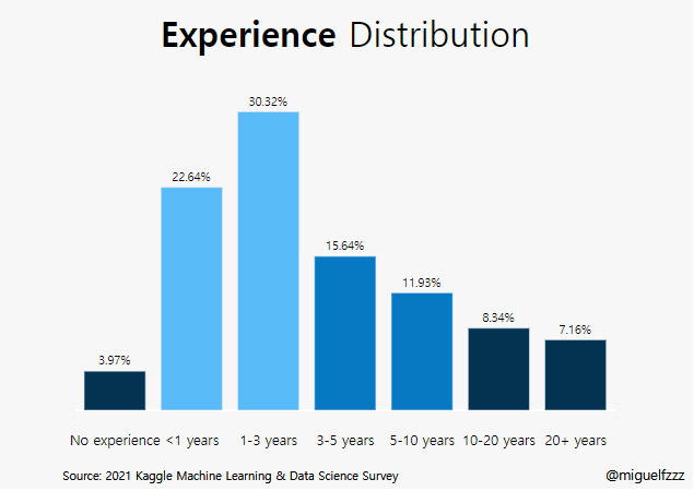
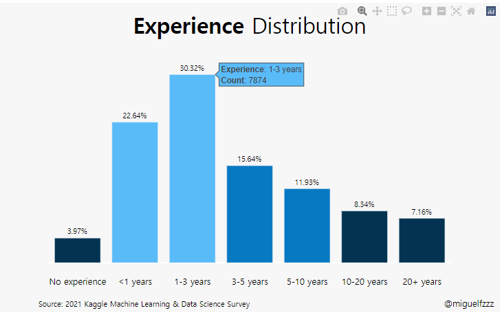
2021-11-08 게시 됨2021-11-09 업데이트 됨13분안에 읽기 (약 1917 단어)

kaggle :Bar Graph (Q6)

kaggle dictation (02)

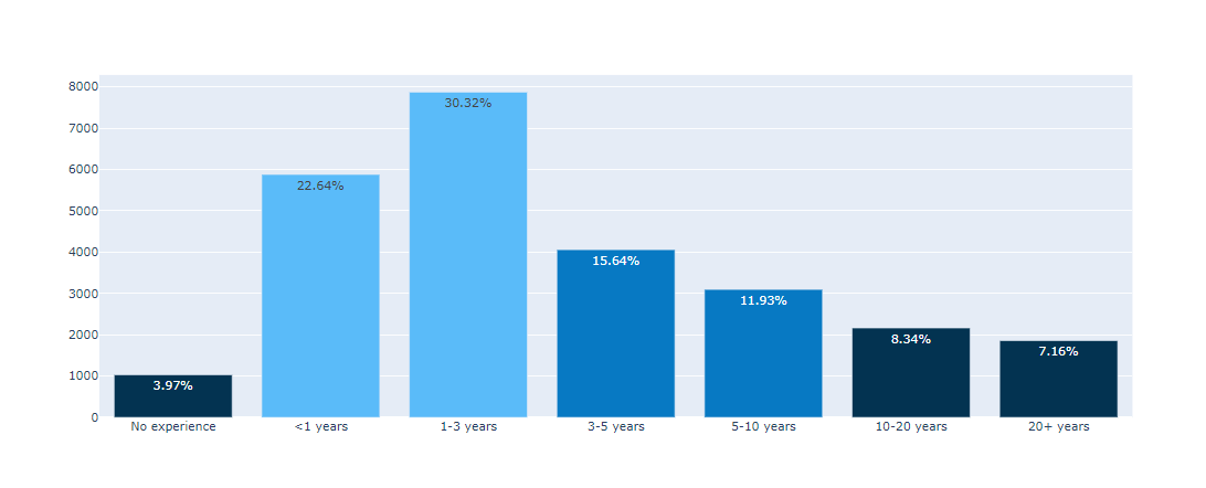
plotly.graph_objects as go: 를 이용한 bar graph

###bar plot /막대 차트

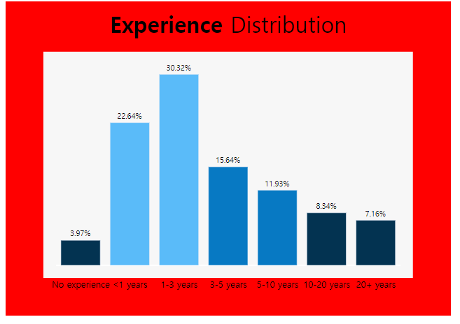
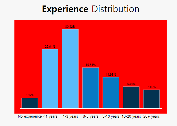
막대그래프는 가장 많이 쓰이는 플롯들중 하나로 숫자 변수와 범주 형 변수 간의 관계를 보여 줍니다.

막대 차트는 종종 히스토그램과 혼동 되기도 하는데(숫자의 분포를 보여줌) 이는 통계학의 부분

그룹당 여러 값이 있는 경우에는 박스플롯이나 바이올린 플롯을 추천

최소한 그룹당 관측치 수와 각 그룹의 신뢰구간은 표시되야함.

사용한 Library

import pandas as pd
import numpy as np
import seaborn as sns
import plotly.express as px
import plotly.graph_objects as go

import warnings
warnings.filterwarnings('ignore')

사실 이 부분에서 seaborn을 사용 했는지 잘 모르겠음.
github에서 plotly가 동적 Livrary라 자꾸 오류가남.

data import

data 원문

data import 방법

data: Kaggle의 the-typical-kaggle-data-scientist-in-2021

이 부분은 data import 방법 을 참고 하거나
kaggle dictation (01) 을 참조하세요.

data encoding (Feature Engineering)

사실 이 부분이 feature Engineering에 해당하는 부분인지 잘 모르겠다.
이 부분은 data를 computer로 자동화하여 계산, 동적 그래프를 만들기 위한 부분.

###Feature Engineering

Experience라는 Question 6에 해당하는 값을 전처리 해 준다.

experience = (
    df['Q6']
    .value_counts()
    .to_frame()
    .reset_index()
    .rename(columns={'index':'Experience', 'Q6':'Count'})
    .replace(['I have never written code','< 1 years',
              '1-3 years', '3-5 years', '5-10 years',
              '10-20 years', '20+ years'], ['No experience', '<1 years',
                                        '1-3 years', '3-5 years', '5-10 years',
                                        '10-20 years', '20+ years'])
          )

.value_counts() : 데이터의 분포를 확인하는데 매우 유용한 함수

column 값의 개수를 확인 하는것. 중복되는 값을 묶어줌.

.to_frame() : frame을 설정 (표 생성)
reset_index()

원본 data를 회손하지 않고 Index를 새로 만듦

.rename(columns={‘index’:’Experience’, ‘Q6’:’Count’})
- column에 새로운 이름을 붙여줌 index는 Experience로 Q6은 count로 지정
replace()
- [왼쪽]에 있는 값대신 [오른쪽]에 있는 값을 넣으려고 함.
- 이 경우 ‘I have never written code’를 ‘No experience’로 바꾸려고 한듯.

Ref. 판다스 함수

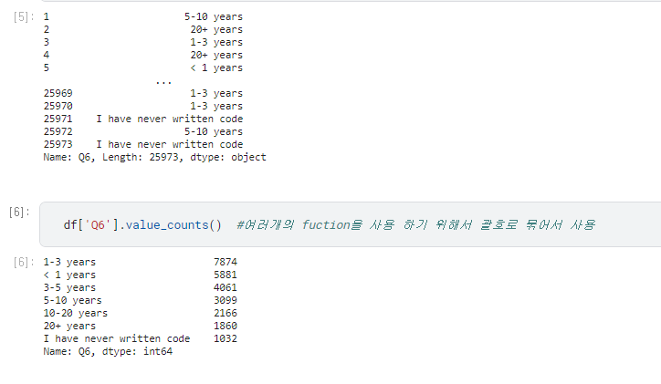
df.value_counts() 함수만 사용하면 아래와 같이 나온다.
1
df['Q6'].value_counts()
1-3 years 7874
< 1 years 5881
3-5 years 4061
5-10 years 3099
10-20 years 2166
20+ years 1860
I have never written code 1032
Name: Q6, dtype: int64

valueCount

이는 문자형 data를 분석하여 display하기 위한 방법

data categoircal로 List로 만들고, 함수정의, 정렬

(#1) : Pandas lib의 categories function

문자열 객체의 배열을 series로 변환하여 범주형으로 변환

#1
experience['Experience'] = pd.Categorical(
                                        experience['Experience'], 
                                        ['No experience', '<1 years',
                                        '1-3 years', '3-5 years', '5-10 years',
                                        '10-20 years', '20+ years']
                                         )

pd.categories

(#2) : experience[‘percent’]

Experience에 하나의 tap을 추가 해준다.
SQL 의 insert 에 percent tep을 만들어 줄 때 column에대해 계산하여 값을 보여주는 것과 같은 느낌.

value에 들어갈 수식 지정_ Experience의 percent 계산

1
2
3

                                         
#2
experience['percent'] = ((experience['Count'] / experience['Count'].sum())*100).round(2).astype(str) + '%'

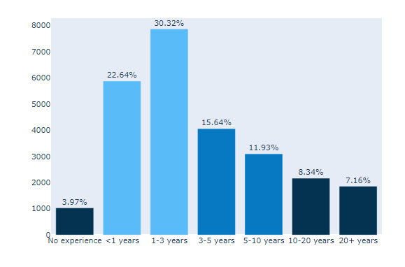
(#3) : experience.sort_values()

데이터 정렬하기 : 컬럼의 data를 기준으로 정렬
- short_Index의 경우에는 Index를 기준으로 data를 정렬한다.
- 이 경우에는 (‘Experience’)를 기준으로 default값인 오름차순으로 정렬

experience.sort_values()

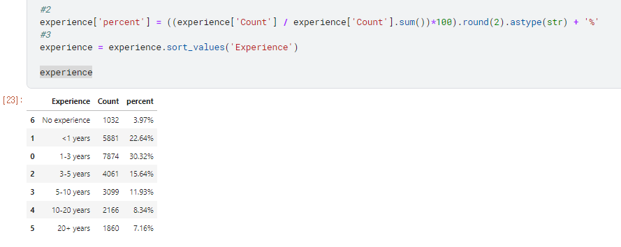
보통 percent나 count를 기준으로 정렬 되는데 이 경우 sort_values(‘Experience’) 를 하였기때문에
기준인 Experience를 기준으로 오름차순으로 정렬 되었다.

Short_value

1
2
3


#3
experience = experience.sort_values('Experience')

(#4) : colors

바chart의 color을 설정

*7 은 7개의 수준이 있다는 것.
colors[N] = 뭘까

chart color


#4
colors = ['#033351',] * 7
colors[1] = '#5abbf9'
colors[2] = '#5abbf9'
colors[3] = '#0779c3'
colors[4] = '#0779c3'

(#5) : fig = go.Figure(go.Bar())

import plotly.graph_objects as go 이기
때문에 fig는 plotly library 함수 사용

#5
fig = go.Figure(go.Bar(
            y=experience['Count'],
            x=experience['Experience'],
            cliponaxis = False,
            text=experience['percent'],
            marker_color=colors
                        ))

x축, y축 정해주기

y=experience[‘Count’],

x=experience[‘Experience’],

cliponaxis

cliponaxis = False,

cliponaxis – Text node를 아래 축에 고정 할지 아닐지 결정
text node를 축 라인과 체크라벨 위에 보여주기위해서는 x축Layer와 y축 layer 설정을 해 주어야 한다.

text=experience[‘percent’]
marker_color=colors
- 지정 해 준 colors를 사용.

(#6) : fig.update_traces()

그래프 위에 캡션 다는 기능

Perform a property update operation on all traces that satisfy the specified selection criteria
지정된 선택 기준을 충족하는 모든 추적에 대해 속성 업데이트 작업 수행 (?? 전혀 모르겠군 !)
아래 본문과는 상관없는 data를 좀 보세요.

df1 = df['Q1'].value_counts()
df2 = df['Q1'].value_counts(normalize = True)
val_pnt_df = pd.DataFrame({"count":df1,"%":df2*100})

fig = go.Figure()
# [str(x) + ' %' for x in np.round(val_pnt_df["%"].values, 1).tolist()]
# Add Traces
fig.add_bar(x = val_pnt_df.index, 
            y = val_pnt_df['count'].values, 
            text = [str(x) + ' %' for x in np.round(val_pnt_df["%"].values, 1).tolist()], 
            textposition="auto")

# layout
fig.update_layout(title_text = "Q1. " + questions[1])

fig.show()

python의 comprehension

오늘은 못보고 나중에 다시 보자 !


#6
fig.update_traces(texttemplate='%{text}', 
                  textposition='outside',
                  hovertemplate='<b>Experience</b>: %{x}<br><extra></extra>'+
                                '<b>Count</b>: %{y}', textfont_size=12)

texttemplate=’%{text}’, : text type
textposition=’outside’, : inside하면 그래프 안쪽, ouside 하면 그래프 위쪽에 생성
hovertemplate= 커서를 가까이 대면 나오는 창 x값과, y 값이 어떤 상태인지 알려 준다.

Experience

hevertemplate

Returns the Figure object that the method was called on

메서드가 호출된 그림객체를 반환.

plotly.graph_objects.Figure.update_traces

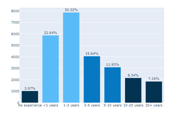
hovertemplate_up

1
2
3

#7
fig.update_xaxes(showgrid=False)
fig.update_yaxes(showgrid=False)

(#7) : fig.update_?axes()

만들어진 fig를 수정.
SQL의 update와 비슷한 기능인듯.

fig.update_xaxes(showgrid=False) : x축의 grid 수정
fig.update_yaxes(showgrid=False) : y축의 grid 수정

showgrid=False

축을 보이지 않는 형태로 바꾸어 예쁘게 보이게 해줌.

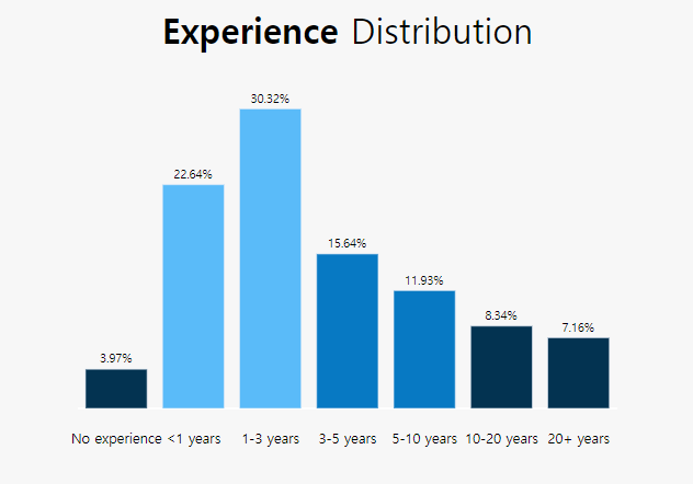
(#8) : update_layout()


#8
fig.update_layout(showlegend=False, 
                  plot_bgcolor='#F7F7F7', 
                  margin=dict(pad=20),
                  paper_bgcolor='#F7F7F7',
                  height=500,
                  yaxis={'showticklabels': False},
                  yaxis_title=None,
                  xaxis_title=None,
                  title_text="<b>Experience</b> Distribution",
                  title_x=0.5,
                  font=dict(family="Hiragino Kaku Gothic Pro, sans-serif", size=14, color='#000000'),
                  title_font_size=35)

default로 되어있는 그래프의 Layout을 수정.

UpdateLayout

showlegend = False
- 래전드를 보여줄지 : 안보여줌
plot_bgcolor=’#F7F7F7’
margin=dict(pad=20)
-dic에는 여러가지가 올 수 있는데 여기서는 dict(pad)를 사용
- padding을 설정, 축과 그래프 사이의 패딩을 px 단위로 설정
- Sets the amount of padding (in px) between the plotting area and the axis lines
- layout-margin
paper_bgcolor=’#F7F7F7’
- 배경색 설정
height=500
- plot size 설정
yaxis={‘showticklabels’: False}
- y축의 showticklabels 설정 : 안함
yaxis_title=None, xaxis_title=None
- y축 제목, x축 제목 설정 : 없음
title_text=”Most Recommended Programming Language“
- 제목 달기 <b> code는 bolde tag인듯.
title_x=0.5, title_y=0.95,
- 제목의 위치 (상단 고정)
font=dict(family=”Hiragino Kaku Gothic Pro, sans-serif”, size=17, color=’#000000’),
```
            title_font_size=35)
```
- title의 font 설정 (Default: “”Open Sans”, verdana, arial, sans-serif”)
- font 설정
- family, color, size 설정 가능, title_fond도 함께 설정 가능 해 보임.

plotly.graph_objects.Figure.update_layout

(#9) : add_annotation()

annotation의 경우 plot 안에 글을 집어 넣는 것.

설명을 추가 해 준다고 생각하면 쉽다.

어렵지도 않고, 같은 내용이므로 이전 posting을 첨부

annotation


fig.add_annotation(dict(font=dict(size=14),
                                    x=0.98,
                                    y=-0.24,
                                    showarrow=False,
                                    text="@miguelfzzz",
                                    xanchor='left',
                                    xref="paper",
                                    yref="paper"))

fig.add_annotation(dict(font=dict(size=12),
                                    x=-0.03,
                                    y=-0.24,
                                    showarrow=False,
                                    text="Source: 2021 Kaggle Machine Learning & Data Science Survey",
                                    xanchor='left',
                                    xref="paper",
                                    yref="paper"))
fig.show()

ref.

plotly.graph_object Parameter

var chart in plotly/en