1
2
3
4
5
6
7
8
9
10
11
12
13
14
15
16
17
18
19
20
21
22
23
24
25
26
27
28
29
30
31
32
33
34
35
36
37
38
39
40
41
42
43
44
45
46
47
48
49
50
51
52
53
54
55
56
57
58
59
60
61
62
63
| import pandas as pd
from sklearn.preprocessing import LabelEncoder
from sklearn.model_selection import train_test_split
import numpy as np
from sklearn.model_selection import StratifiedKFold
from sklearn.linear_model import LogisticRegression
from sklearn.pipeline import make_pipeline
from sklearn.preprocessing import StandardScaler
from sklearn.decomposition import PCA
import matplotlib.pyplot as plt
from sklearn.model_selection import learning_curve
from sklearn.model_selection import validation_curve
from lightgbm import LGBMClassifier
data_url = 'https://archive.ics.uci.edu/ml/machine-learning-databases/breast-cancer-wisconsin/wdbc.data'
column_name = ['id', 'diagnosis', 'radius_mean', 'texture_mean', 'perimeter_mean', 'area_mean', 'smoothness_mean', 'compactness_mean', 'concavity_mean',
'concave points_mean', 'symmetry_mean', 'fractal_dimension_mean', 'radius_se', 'texture_se', 'perimeter_se', 'area_se', 'smoothness_se',
'compactness_se', 'concavity_se', 'concave points_se', 'symmetry_se', 'fractal_dimension_se', 'radius_worst', 'texture_worst', 'perimeter_worst',
'area_worst', 'smoothness_worst', 'compactness_worst', 'concavity_worst', 'concave points_worst', 'symmetry_worst', 'fractal_dimension_worst']
df = pd.read_csv(data_url, names=column_name)
X = df.loc[:, "radius_mean":].values
y = df.loc[:, "diagnosis"].values
le = LabelEncoder()
y = le.fit_transform(y)
X_train, X_test, y_train, y_test = train_test_split(X, y, test_size = 0.20,
random_state=1)
kfold = StratifiedKFold(n_splits = 10, random_state=1, shuffle=True)
pipe_lr = make_pipeline(StandardScaler(),
PCA(n_components=2),
LogisticRegression(solver = "liblinear", penalty = "l2", random_state=1))
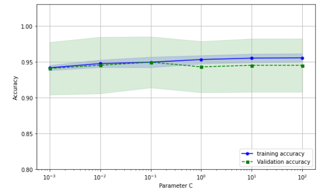
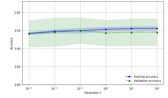
param_range = [0.001, 0.01, 0.1, 1.0, 10.0, 100.0]
train_scores, test_scores = validation_curve(estimator=pipe_lr,
X = X_train,
y = y_train,
param_name = "logisticregression__C",
param_range = param_range,
cv = kfold)
train_mean = np.mean(train_scores, axis = 1)
train_std = np.std(train_scores, axis = 1)
test_mean = np.mean(test_scores, axis = 1)
test_std = np.std(test_scores, axis = 1)
fig, ax = plt.subplots(figsize = (16, 10))
ax.plot(param_range, train_mean, color = "blue", marker = "o", markersize=5, label = "training accuracy")
ax.fill_between(param_range, train_mean + train_std, train_mean - train_std, alpha = 0.15, color = "blue")
ax.plot(param_range, test_mean, color = "green", marker = "s", linestyle = "--", markersize=5, label = "Validation accuracy")
ax.fill_between(param_range, test_mean + test_std, test_mean - test_std, alpha = 0.15, color = "green")
plt.grid()
plt.xscale("log")
plt.xlabel("Parameter C")
plt.ylabel("Accuracy")
plt.legend(loc = "lower right")
plt.ylim([0.8, 1.03])
plt.tight_layout()
plt.show()
|