DecisionTreeMachineLearning(03)
machine Learning Model Algoridms
- 비 선형 모델 : KNN,
- 선형 모델 :
Decision Tree MachineLearning
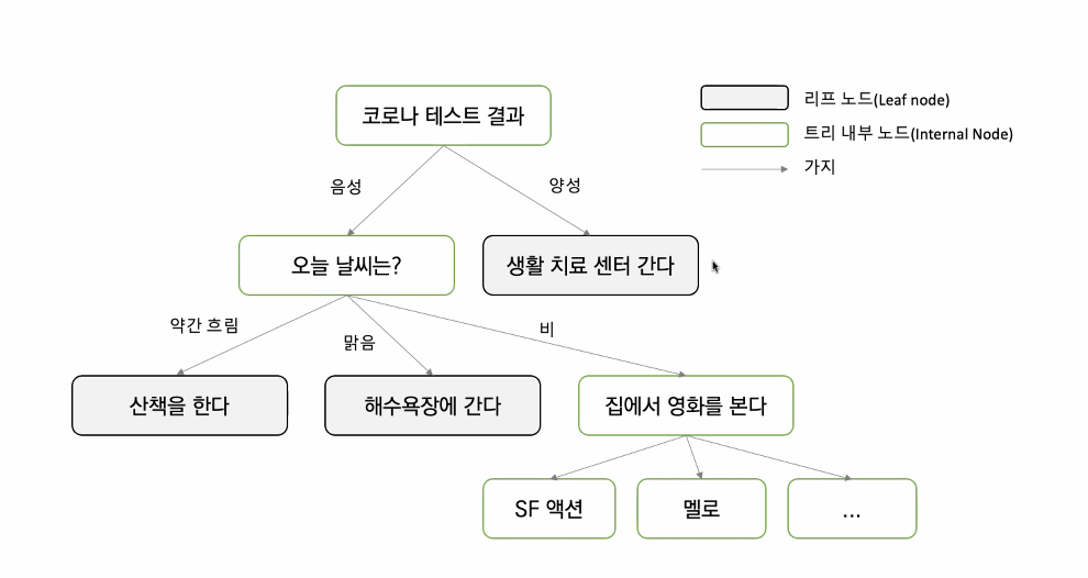
Introduction
- 과적합 : 모델의 정확도만 높이기 위해 분류 조건(depth)만 강조하여 실제 상황에서 유연하게 대처하는 능력이 떨어지게 되는 문제가 발생하게 되는것.
- 가지치기(pruning)을 통해 유연성을 유지.
- Max_depth를 대략적으로 잡아서 (3, 5, 10…) RMS 값 비교
- Random search
- 하이퍼파라미터 (grid Search)
분류기준 (수식은 아래서 책에서 확인)
- 정보이득 :
- 자식노드의 불순도가 낮을 수록 정보의 이득이 커진다.(효율성 Up)
- 정보 이득이 높은 속성을 기준으로 알아서 나누어 준다.
- 엔트로피의 정의 :
- 엔트로피는 높을 수록 좋다.
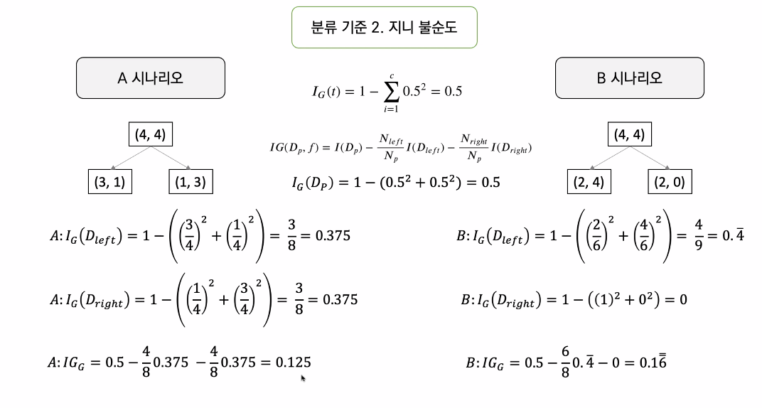
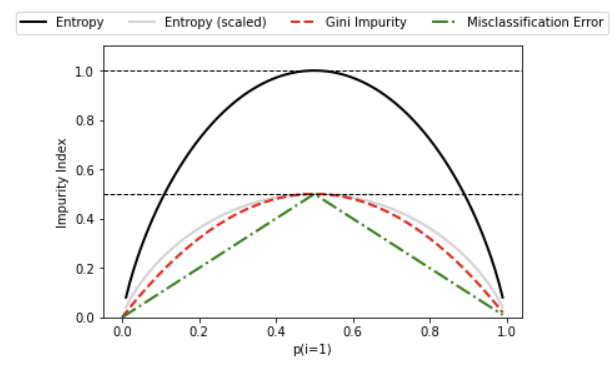
- 지니불순도 :
- 순도는 높을 수록 좋다.
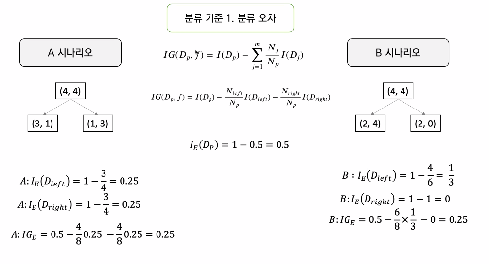
- 분류오차 :
- 어떤 시나리오가 더 좋은가에 대한 계산
- 1이 되면 균등, 완벽하게 나누어 졌다고
- 정보이득 :
ㅇㅇ
공식은 이쪽에 가면 있다.
계산은 컴퓨터가 다 해준다.
우리는 보고 좋은 분류 기준을 선택 하며 됩니다.
분류기준 1. 분류 오차
분류기준 2. 지니 불순도
분류기준 2. 엔트로피
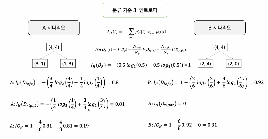
- 정보이득을 최대로 하는 옵션을 찾는다.
실습
1 | from sklearn import datasets |
클래스 레이블: [0 1 2]
1 | from sklearn.model_selection import train_test_split |
y 레이블 갯수: [50 50 50]
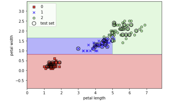
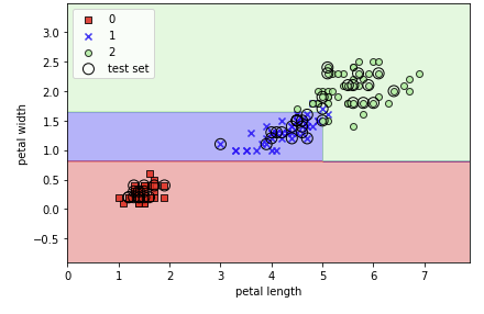
시각화
1 | from matplotlib.colors import ListedColormap |
1 | import matplotlib.pyplot as plt |
- 정보 이득을 최대로 하는 옵션을 찾아서
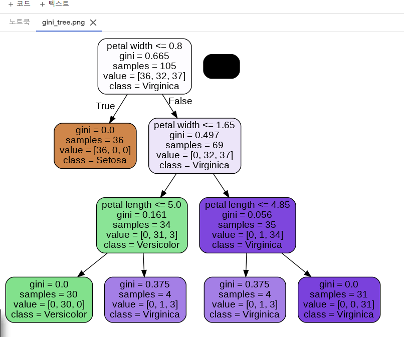
1 | from sklearn.tree import DecisionTreeClassifier |
DecisionTreeClassifier(max_depth=3)
- depth를 3으로 해 주었기 때문에 과적합 X
1 | X_combined = np.vstack((X_train, X_test)) |
1 | from pydotplus import graph_from_dot_data |
True
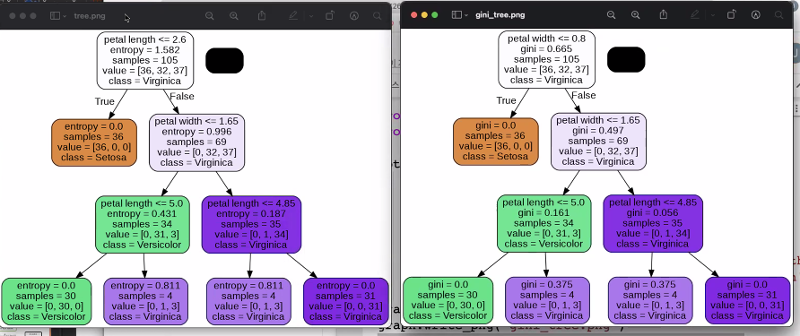
- gini 로 1개 Entripy 로 1개 짜서 해야함
gini: defaultEntropy: 도 해보고 비교
1 | tree_entropy = DecisionTreeClassifier(criterion="entropy", max_depth=3) |
- 모형을 도식화로
1 | from pydotplus import graph_from_dot_data |
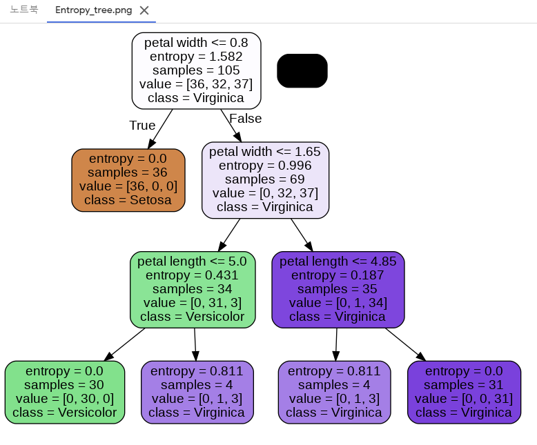
entropy가 0이 되면 더이상 나눌 필요가 없다.
- sklearn에서는 분류오차는 없다.
- 지니 와 엔트로피 두개를 보고 더 나은 것을 선택
<아직 안배운 부분>
- 스태킹 알고리즘 (앙상블)